Volume 11, Issue 2, 1997
Microfit 4.0 for DOS: A Review
- Guy Judge and R.I.D. Harris
- University of Portsmouth
Introduction
Since it first appeared nearly a decade ago (originally under the name of DataFIT) the interactive econometric software package Microfit, designed and written by Professors Hashem and Bahram Pesaran, has provided an excellent vehicle for both learning and practising the art of modern applied time series econometrics, and many students, teachers, researchers and professional economists have been able to benefit from it. Structured around a series of interlocking menus, with on-line help and a very clear a ccompanying manual, the program set new standards of user-friendliness and ease of use. It could also be relied upon to include a comprehensive range of estimation and testing procedures for time series econometric modelling, including those which had onl y recently been established in the literature.When version 3.0 of the program came onto the market in 1991 it already incorporated a procedure for estimating cointegration relationships using Johansen's (1988) maximum likelihood method, as well as an ADF command for augmented D ickey-Fuller unit root tests and many other techniques for estimating and testing linear and non-linear dynamic models (see McAleer and Oxley (1993) and Harris (1994)). However both econometrics and technolog y move on, and many users have been eagerly awaiting the new version 4.0 of the package which, it was promised, would incorporate new developments in univariate and multivariate time series analysis and take advantage of the flexibility of the Windows ope rating environment. The DOS version of the new Microfit 4.0 has now been released, and although users must wait a little longer for the Windows version of the product to appear they can get an idea of what to expect if they download a demo version from the Microfit web site.
The new program comes on a CD-ROM (or diskettes on request) and is easy to install. There is a 500 page manual "Working with Microfit 4.0: Interactive Econometric Analysis" which, as well as containing reference material on the program's menus and command s, includes 76 tutorial lessons using more than 25 different real data sets and this provides an excellent introduction or refresher course on modern time series econometric modelling techniques and methodology. This is a most valuable part of the package - for students perhaps the most valuable part - and it will be a great help both to individual learners and to those who teach applied econometric modelling courses built around the use of Microfit.
Data Management
A new companion data access package for Microfit called DETS (Data Extractor for Time Series) - not reviewed here - has been written by Brian Holley, the senior computer computer officer in the Faculty of Economics and Politics at Cambridge. This p rogram has been developed because many Microfit users make use of data extracted from large time series databases such as CITIBASE, Penn World Tables, OECD data, World Bank and ONS databanks. DETS works with its own special internal format and published databases can be converted from their source form into this special format which is compact, and contains an internal index to enable rapid searches to be made. Conversion programs for sources not currently supported may be developed as required. Microfit 4.0 itself will read in data in a variety of formats. As well as its own format (.FIT files) the new version of the program recognises ASCII, TXT and Lotus print (.PRN) files , standard comma delimited (.CSV) files, Excel (version 4.0) worksheets and Aremos (.TSD) files. All files created using Microfit 3 can be used with Microfit 4.0. You can also simply enter data at the keyboard if you wish. Data can be saved in in .FIT, .CSV and .TSD format.
New features
Microfit 4.0 has added a few new functions to those available in version 3 (including the Hodrick and Prescott Filter), a couple of new commands for reordering observations according to the size of one of the variables (mainly relevant for the analysis of cross-section data) and many new single equation and system equation options.New single equation options include LOGIT and PROBIT estimation procedures, the Phillips-Hansen Fully Modified OLS method of estimating cointegrating relations, and a procedure for using model selection criteria to estimate a single cointegrating relation within an Autoregressive-Distributed Lag (ARDL) framework. The approach allows for the inclusion of time trends, seasonal dummies and other deterministic/exogenous regressors in the cointegrating relation. There is a whole raft of maximum likelihood pro cedures for the estimation of models under various conditional heteroskedastic error specifications (likely to be particularly relevant in finance applications). The program also offers new procedures for non-nested tests of linear versus log-linear model s (in level differenced and log-differenced form) and also for some other non-linear specifications of the dependent variable.
The program now has a comprehensive set of options for estimating and testing multiple equation (systems) models covering unrestricted VAR models, cointegrating VAR models and Seemingly Unrelated Regression (SURE) models, in both unrestricted and restrict ed form. Akaike, Schwarz and log-likelihood criteria are available to assist in the selection of a suitable model. There are procedures for new cointegration tests in VAR models and the analysis of identifying and overidentifying restrictions on the lo ng-run cointegrating relations. The computation of orthogonalized and generalized impulse response functions, multivariate dynamic forecasts, and forecast error-variance decomposition is also possible with the Microfit 4.0.
Figure 1 gives an overview of the menus structure of the new program.
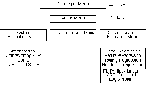
Figure 1: A flow chart of the menus in Microfit 4.0
Click to see the full size graphic
Example to illustrate the look and feel of Microfit 4.0 for DOS
Thomas (1997) uses Microfit 3.0 to estimate and test a simple dynamic model of the demand for food using aggregate US time series data (data set 1 on the floppy disk accompanying his book). To illustrate the way that Microfit 4.0 looks and operates, and to compare the output from the new version with that of version 3 (which is printed on pages 364 and 365 of Thomas's book) we will now work through this example step by step.First, a brief comment about the data. It consists of annual data from 1963 to 1992, taken from the OECD National Accounts. The variables in the file are as follows:
NF	 = 	expenditure on food in current prices
RF	 =	expenditure on food in constant (1980) prices
NTE	 =	total expenditure in current prices
RTE	 = 	total expenditure in constant (1980) prices
Thomas treats RF = Q as a measure of food demand, NTE = X as a measure of total consumers' expenditure, NF/RF = P is an index of the price of food and NTE/RTE = G is a general price index. The computer exercise requires one to begin by estimating a model with log Q as the dependent variable and the logs of X, P and G, together with one period lags of all variables (including the dependent variable) as regressors.
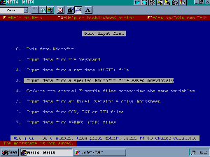
Figure 2: Data Input Menu
Click to see the full size graphic
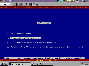
When you run Microfit 4.0, after a brief copyright screen you arrive at the Data Input Menu (see Figure 2). The program positions you over option 3, ready to load up data from a Microfit file, but if you want to use a file in one of the other acceptable f ormats or enter new data at the keyboard you can select one of the other options.
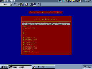
Figure 3: File Selection Box
Click to see the full size graphic
Figure 4: Action Menu
Click to see the full size graphic
A box opens allowing you to move through the various drives and directories available to you until you locate the file you want (see Figure 3). You are then taken to the Action Menu (Figure 4) where you can either procede directly to another menu and esti mate a single equation or multivariate model, or, as we do here, select option 1 so that we can transform the series in the data file into the ones we want to work with in our analysis.
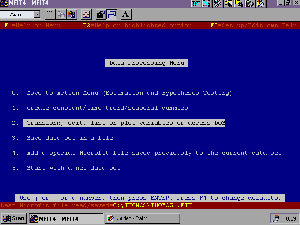
Figure 5: Data Processing Menu
Click to see the full size graphic
Figure 6: Formula and Commands Screen Editor
Click to see the full size graphic
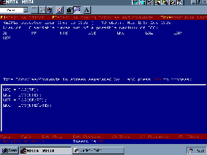
Next you are taken to the Data Processing Menu (Figure 5) where we select option 2. A screen editor then appears (see Figure 6) with a box at the bottom where you enter formulae or commands. The variables currently in the memory will be listed at the top. Here you see the screen after the formulae have been entered and computed. You can also see that Help is available by pressing F1 or F2 as required. At this stage you might wish to examine the data graphically and there are commands to produce time serie s plots or scatter diagrams of variables. On leaving this screen editor (by pressing Esc) you are taken back to the Data Processing menu. Note that the program requires you to create your own constant intercept term so you should do this first before movi ng back through the Action Menu and on to the Single Equation Estimation Menu (Figure 7).
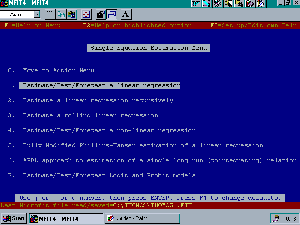
Figure 7: Single Equation Estimation Menu
Click to see the full size graphic
Figure 8: Model Specification Screen Editor
Click to see the full size graphic
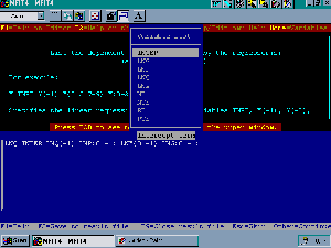
Here we select option 1 and this takes us on to the model specification screen editor. Figure 8 shows how you specify the equation to be estimated. If you forget the names of any of the variables you can press the Home key to get a drop down menu with a full variable list, as shown here. On leaving this box you will be prompted for the estimation period to use. Just pressing
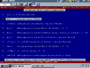
Figure 9: Estimation Menu (Linear Regression)
Click to see the full size graphic
Figure 10a: OLS Results
Click to see the full size graphic
Figure 10b: Regression Diagnostics
Click to see the full size graphic
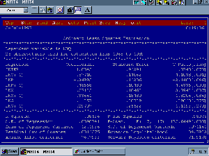
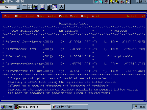
Next you select the estimation method (see Figure 9) and the results will then appear on the screen as shown in Figures 10a and 10b. The main results table is very similar to that produced by Microfit 3.0, except that it now includes the Akaike Informatio n Criterion (AIC) and Schwarz Bayesian Criterion statistics.
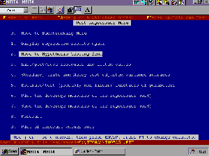
Figure 11: Post Regression Menu
Click to see the full size graphic
Figure 12: Hypothesis Testing Menu
Click to see the full size graphic
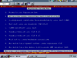
At this stage the results may either be printed or saved to disk, after which you are taken to the Post Regression Menu (see Figure 11). Moving to the Hypothesis Testing Menu you can choose from a variety of specification and misspecification tests (see F igure 12). Moving via the Post Regression Menu you can then go to a menu (Figure 13) where you can examine the residuals or fitted values graphically, or save them to disk.
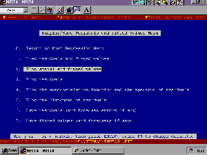
Figure 13: Display/Save Results and Fitted Values Menu
Click to see the full size graphic
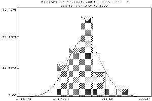
Figure 14: Residuals Histogram
Click to see the full size graphic
Figure 14 shows what the histogram of the residuals looks like in this case. The screen display is in colour, but before saving the graphic image (in one of a number of different formats) you can switch to a monochrome version by just pressing any key on the keyboard. This a very quick and convenient feature.
We will leave this example at this point as it should be enough to illustrate the look and feel of the program and to show how the program operates. Thomas's example goes on to test the suitability of various restricted formulations nested within the orig inal model and this is easily accomplished within Microfit. Alternatively, in this case one could have made use of the new ARDL procedure described below
Cointegration Analysis with Microfit 4.0
As noted before, Microfit 4.0 includes an extensive range of facilities for cointegration analysis. For single equation models with I(1) exogenous variables one can use the Phillips-Hansen (1990) fully-modified OLS procedure to est imate the equation's parameters. (This is an extension of the Engle-Granger method which takes account of possible correlations between the disturbances in the cointegrating regression and the processes driving the exogenous variables and allows for the p ossibilty of a deterministic trend in the cointegrating relations.) Alternatively you can search for a suitable specification from within an Autoregressive-Distributed Lag (ARDL) model, using the Akaike Information Criterion, the Schwarz Bayesian Criterio n, the Hannan-Quinn criterion to help you select the maximum lags required for each variable. Even with quite a small number of exogenous variables and low maximum lag lengths this can mean that quite a large number of separate regressions have to be esti mated and it may take a few minutes to get the final results; Microfit 4.0 helpfully provides a warning message before this process is initiated. Both the Error-Correction representation and the long-run/steady-state equation (with asymptotic standard er rors for the estimated coefficients) can be displayed. Although we have our doubts about using this automated procedure for model selection it can at least provide a benchmark against which to compare your own preferred model.Where there is likely to be more than one cointegrating vector it is necessary to approach the analysis from a system or multiple equation perspective and Microfit 4.0 implements a generalization of the Johansen Maximum Likelihood procedure within the fra mework of a vector error correction model (VECM). The model allows for the inclusion of a number of I(1) exogenous variables and intercept and deterministic trend terms. The endogenous and exogenous variables are separated by an ampersand sign (&) i n the list entered into the cointegration analysis editing box, but the user must choose from a menu the combination of intercept and deterministic trends to allow for.
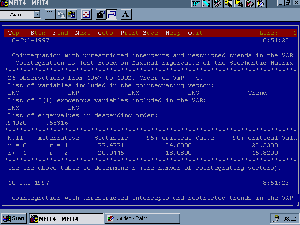
Figure 15: Cointegration Results showing Maximal Eigenvalues
Click to see the full size graphic
A set of results for each endogenous variable is then presented, giving the trace and maximum eigenvalue statistics for testing hypotheses concerning the rank of the long-run matrix, together with critical values at the 90 and 95% levels. (See Figure 15. Note: these are based on those computed by Pesaran et al. 1996, rather than the original Johansen-Juselius or Osterwald-Lenum values.) The program also gives you the maximized values of the log-likelihood function of the cointegrat ing VAR model, Akaike, Schwarz, and Hannan-Quinn model selection criteria for the different values of r.
Before you can proceed you must choose a value of r. Sometimes the criteria all point to the same value for r but in other cases (including the example used in the tutorial) there may be a conflict and it will be necessary to turn to relevant economic th
eory for assistance. One this is done you can view the cointegrating vectors and the matrix of long run multipliers (but not, unfortunately, the speed of adjustment coefficients ![]() ). You can then go on to
test restrictions on the cointegrating vectors i.e. the long-run parameters (but again it is not possible to test restrictions on
). You can then go on to
test restrictions on the cointegrating vectors i.e. the long-run parameters (but again it is not possible to test restrictions on ![]() and hence weak exogeneity). If the identifying or over-identifying restr
ictions are applied the program presents the (normalized) cointegrating vectors with the standard errors. Restictions to be tested are entered in simple form in a dialog box and can be saved in a file for later use.
and hence weak exogeneity). If the identifying or over-identifying restr
ictions are applied the program presents the (normalized) cointegrating vectors with the standard errors. Restictions to be tested are entered in simple form in a dialog box and can be saved in a file for later use.
Concluding remarks
The new version of Microfit brings the program up to date by including many new procedures and incorporating some of the latest refinements into existing routines, to produce what is a very powerful tool for modern interactive econometric modelling. There are some improvements in the operation of the program through its menus and screen input boxes, but until the Windows version is available some users may feel that it lags behind its competitors in terms of ease of use. The manual which accompanies the p rogram is well put together and the tutorial lessons which are based on real data sets and well-known studies from the literature provide a valuable learning resource.
References
Harris, R.I.D. (1994) Cointegration Analysis Using the Johansen Technique: A Practitioner's Guide to the Software. The Economic Journal, Vol 104 pp 1227-1237.Johansen, S. (1988) Statistical Analysis of Cointegration Vectors. Journal of Economic Dynamics and Control, Vol 12 pp 231-254.
McAleer, M. and Oxley L. (1993) Microfit 3.0. An Interactive Econometric Software Package. The Economic Journal, Vol 103 pp767-774.
Pesaran, M.H., Shin, Y. and Smith, R.. (1996) Structural Analysis of Vector Error Correction Models with Exogenous I(1) variables. Unpublished manuscript, University of Cambridge.
Phillips, P.C.B and Hansen B.E. (1990) Statistical Inference in Instrumental Variables Regression with I(1) processes. Review of Economic Studies, Vol 57 pp99-125.
System Requirements
IBM PC (or fully compatible) with 80386, 80486 or Pentium processor with- at least 4Mb free RAM (8Mb recommended)
- DOS 3.0 or higher
- at least 12 Mb of free hard disk space
- VGA or SVGA monitor
Pricing and ordering information
Prices vary according to the type of user (commercial/academic/student), the number of copies purchased (site licences are available) and the geographical location of the user. There are special prices for users of Microfit 3.0 who are upgrading. To give a few examples, in the UK an academic site licence is Ł950, a commercial site licence is Ł1900 and a student version is Ł60 (all excluding VAT). Additional copies of the manual cost Ł25.For further information, or to order the software contact either Oxford University Press (United Kingom and the rest of the world except USA, Canada and Mexico) or Camfit Data Limited (USA, Canada and Mexico) at the addresses below:
Janet Caldwell,
Customer Service Department, Electronic Publishing, Oxford University Press, Walton Street, Oxford OX2 6DP; United KingdomTelephone +44 1865 267979
Fax +44 1865 267990
E-mail CALDWELLJ@OUP.CO.UK
Mrs Marian Swainston,
Camfit Data Limited, 283 Hills Road, Cambridge CB2 2RP, United KingdomTelephone +44 1223 500639
Fax +44 1223 564 379
E-mail CAMFIT@SERVER1.INTECC.CO.UK
Alternatively go the Microfit World-Wide Web site from where order forms can be downloaded.
Editor's Note: Just as this issue of CHEER was going to press we received a copy of the Windows version of Microfit 4.0 We will provide an update review in a future issue.


