Volume 12, Issue 1, 1998

Long-Run Dynamic Market Equilibrium Simulation through the use of Spreadsheets
- Holger Paetow
- Hochschule für Wirtschaft und Politik, Hamburg
1 Introduction
Modern computer technology has expanded the range of complexity and sophistication in economic research and teaching alike. This particularly applies to high performance graphic modules for spreadsheet programs, where excellent graphics properties, are combined with user friendly high performance calculation capabilities. It seems a far more effective method of teaching students, by using a multi-purpose instrument like EXCEL to analyze economic problems, than to work with specialized economic teachware.
To illustrate the scope of this type of approach, an example will be presented to show the possibility of changing parameters and increasing the complexity of the model in a 3-d-display with “real-time” variations. The implementation of the model with a spreadsheet program such as EXCEL 97, should not be very difficult for someone with a reasonable grasp of the program. For this reason it is not necessary to elaborate on the spreadsheet entries in detail.
2 Basic Model
In neoclassical theory, long-term market equilibrium exists in an area where prices, quantities and number of suppliers of different sizes all move simultaneously. This occurs under the premise of free market entry, and varying plant size. This is normally shown in conventional teaching material in a static-comparative mode applied to aggregates. The analysis and graphical illustration of market forces has always been difficult, because of the simultaneous reaction of various actors, and the complexity of related movements. This can be noted particularly when plant size variations lead to economies of scale.
2.1 Assumptions
The model shown here is based on the following assumptions. The market has 20 suppliers of varying plant size (output capacity). All suppliers automatically adjust plant capacity depending on the profits of the preceding period.
(1) ![]()
where
xit,xit-1 : maximum output capacity of the i-th supplier in t and t-1 respectively
![]() : profits of the
i-th supplier t-1
: profits of the
i-th supplier t-1
XA : capacity adjustment factor (which indicates that the change in capacity is proportional to profits)
Should the capacity of a firm sink below xmin then the capacity of the following period will be adjusted to zero. This serves to illustrate the exit of a firm from the market where loss of market share and therefore profits reflect inability to compete. Market entry is not envisaged in this model.
The individual short-run total unit costs(1) are linear functions of output quantity.
(2) Cit = aC + bC • qit
and
(3) ![]()
where
Cit : total costs of the i-th supplier in period t
cit : unit costs of the i-th supplier in period t
qit : sales of the i-th supplier in period t
aC, bC parameters of the cost function
Increasing plant size leads to rising fixed costs while the marginal costs decline. Therefore in this model it is assumed that aC and bC are in a direct arithmetic-linear relationship to variations of plant size.
(4) aC = aaC + baC • xit
(5) bC = bbC + bbC • xit
where
aaC, baC, abC, bbC are parameters which adjust short-run cost function to plant size
Total demand is a linear function of market price
(6) Dt = aD + bD • Pt
where
Dt : total demand in period t
Pt : market price in period t
aD, bD : parameters of the demand function
Products are homogenous in the basic model and therefore a uniform market price Pt applies. Plant capacity dictates markets share for the suppliers up to the point where their maximum plant capacity has been achieved. With linear short-run cost functions profits are maximized when output is at maximum capacity. Therefore each firm‘s demand will be completely satisfied as long as it does not exceed capacity.
(7) 
where
xit : capacity of the i-th supplier in period t
Xt total capacity of all
suppliers in period t ![]()
Suppliers adjust prices to reflect plant size in the following manner: The change of the market price from period t-1 to t is assumed to be proportional to the difference between total capacity and total demand in t-1. Hence
(8) ![]()
where Spindicates the intensity of price change. P1 the price in the first period t1 can be set at an appropriate level.
The profit level ![]() of the
i-th supplier in period t is determined by
of the
i-th supplier in period t is determined by
(9) ![]()
2.2 Specification of parameters
Firstly the relationship of plant size to the cost functions should be established. This is done through the determination of the parameters aaC, baC, abC, bbC as follows(2):
aaC = 0
baC = 5
abC = 50
bbC = -0,004
The effects can be seen in Fig. 1.
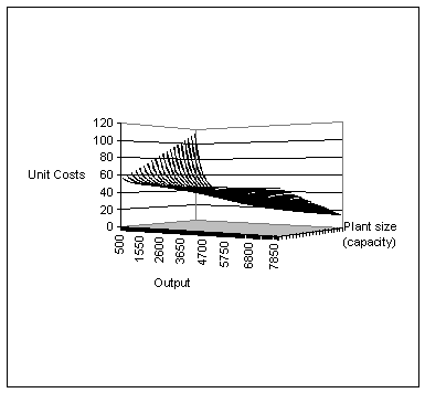
Figure 1: Unit cost functions
Figure 1 depicts the unit cost functions of 20 firms ordered by the level of plant capacity, i.e. the firms with low capacity are to the front and with increasing capacity the firms are regulated to the back.
Given any plant size, the costs per unit sinks with increasing output. In accordance with the previous assumptions, fixed costs are increasing and marginal costs are decreasing with plant size. So compared to larger firms, smaller ones have lower unit costs at lower output level, and are less efficient at higher output level. Increases and decreases in capacity are determined as follows: In the period t1 the plant capacity of the smallest supplier is set at 600. The plant capacities of the other firms are assigned in steps of fifty upwards, so that the largest suppliers (i=20) would have an initial capacity of 1550. In addition XA = 3000 and xmin = 400. That means that for every 3000 units of profit, the plant capacity automatically increases by 1. All suppliers whose capacity sinks below 400 exit the market.
The demand function is as follows:
(6a) Pt = 400-0,005Dt
Sp is set at 1000, the initial price P1 is 80 units and XA is set at 2000.
2.3 Market process in the basic model
As is to be expected the following global trends can be discerned. The
initial total plant capacity is not sufficient to satisfy demand at a
price of 80. (X<D; Xexcess<0,
i.e. under capacity; cf. figure 2). Therefore the price rises generate
profits which are reinvested. This in turn is reflected in increased plant
capacity. Parallel to this demand drops. At a particular point excess
capacity occurs, price is forced down and capacity growth slows because of
diminishing profits. By the end of the experimental run total plant
capacity and demand are in equilibrium (Xexcess
![]() 0).
Price and demand are stable.
0).
Price and demand are stable.
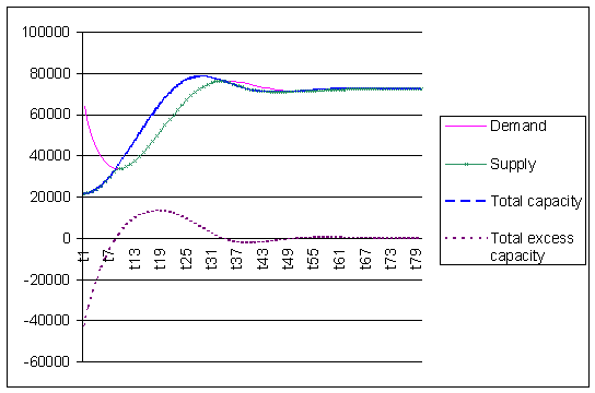
Figure 2: Total demand, total (excess) capacity(3)

Figure 3: Price
The figures 4 and 5 show the evolution of plant capacity, and unit costs of the individual suppliers. This shows that plant capacity increases, are mainly occurring in plants with initial higher capacity. Plants with low capacity display negative growth, as of the period t37. The market structure tend towards concentration.
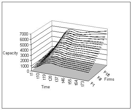
Figure 4: Capacity of individual firms
For obvious reasons the drop in prices due to temporary excess capacity (as of the period t10) cannot be compensated for by cost reductions. Growth is not possible at the speed needed to recoup losses by availing of the economies of scale. This is shown clearly in figure 5.
As time progresses, unit costs fall on the one hand due to price related demand increase, which allows all firms better capacity utilization. On the other hand unit costs decline, particularly with larger firms which from the start have been favored by economies of scale, and are reinvesting their larger profits in fast capacity growth. The smaller firms are forced to reduce plant size due to losses which began as of the period t8 and are therefore less efficient because they lack the ability to optimize economies of scale

Figure 5: Unit costs
3 Extensions of the basic model
3.1 Variation of parameters and time range
This approach presents the possibility of varying all parameters. The above described process of market equilibrium, is relatively less sensitive to changes to the initial price, capacity related factors and other parameters, as long as the values are chosen with a minimum of care. At approximately the same point equilibrium price and equilibrium total capacity are attained. Change in market structure will always follow the same pattern. The initial market structure could be described as oligopoly with mild plant capacity differences. It is of course possible to vary market structure e.g. tight partial oligopoly with three to five large firms, and on the fringe, a group of several smaller competitors, a scenario which often occurs.
3.2 Alternative types of function
If one assumes lower values for XA meaning that reinvested profits lead to a higher capacity growth(4), then at this point the effectiveness of the model is limited, because the basic premise on which the model has been developed is questioned .
Particularly the linear nature of the relationship between cost advantage, and plant capacity growth, could lead to implausible unit cost values, and explosive profit growth. This can be compensated by integrating a quadratic term into the equation (5) e.g. with a value of 0,000001.
(5a) bC = abC + bbC • xit + cbC • xit2
This reflects the results of statistical research, which demonstrate that only up to the point of minimum efficient scale (MES), unit costs can be sunk to avail of the economies of scale. In the case of firms with larger plant size, unit costs remain constant and cannot become negative.
Figures 6 through 9 are similar in content to figures 2 through 5 They demonstrate the market process in a more drastic manner, simply by changing parameters as follows:
- value for XA is only 800,
- cost function as previously described
- an extended time range
Under these conditions the market stabilizes, after initial turbulence, when a much smaller group of similarly sized oligopolists are shown to have survived.
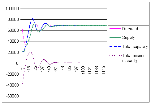
Figure 6: Demand and total (excess) capacity
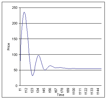
Figure 7: Prices
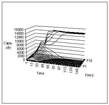
Figure 8: Plant capacity of individual firms

Figure 9: Unit costs (5)
3.3 Additional variations of the model
Besides changing of parameters, it is possible to construct other models, and to further vary existing ones, on completely different assumptions to the basic model. The assumption of a perfectly non-elastic demand, or fixed price state regulation, are comparatively easy to implement by fixing the appropriate parameter at zero. It is a more time consuming exercise to demonstrate the effects of market entry by the incorporation of dummy variables on a random basis, as a result of plant capacity utilization or depending on profit level. This variation of the model allows for a simulation of the market process in a contestable market(6).
Apart from these factors, there are no limits to the number of variations which can be achieved by the manipulation of endogenous and exogenous variables. The demand function can be linked to long-term trends or business cycles. Costs can be made dependent, on time or profit related savings, due to autonomous or induced technical progress. This can further enhance visualisation of the dynamic nature of competition. For a realistic application of this approach, it is particularly important to allow for product differentiation, to enable firm related prices to be analyzed.
Note: The author may be contacted by e-mail
at
PaetowH@hwp.uni-hamburg.de
Footnotes
(1) This reflects the difference between short and long-run costs functions which have applied since Viner, Cost Curves and Supply Curves, Zeitschrift für Nationalökonomie, Vol. III 23 ff.
(2) Parameters are not derived from direct empirical research, rather they are chosen to reflect realistic cost functions.
(3) It should be noted that up to t9 sales cannot exceed capacity. After the period t9 sales are restricted by demand, which reflect in the meeting of supply and demand curve.
(4) e.g. because of lower prices for investment goods which allows the firm to enlarge capacity
(5) Vertical lines are caused by suppliers being forced to exit the market and the model readjusting
(6) cf. W. J. Baumol, J. C. Panzar, R. D. Willig, Contestable Markets and the Theory of Industry Structure, New York 1982
|
What's Related: · Other articles on the use of spreadsheets in teaching economics |

