


The study of economics does not seem to require any specialised gifts of an unusually high order. Is it not, intellectually regarded, a very easy subject compared with the higher branches of philosophy and pure science? Yet good, or even competent, economists are the rarest of birds. An easy subject at which few excel! The paradox finds its explanation, perhaps, in that the master-economist must reach a high standard in several different directions, and must combine talents not often found together.J M Keynes [in Johnson, E and D Moggridge (Eds) (1976): The Collected Writings of J M Keynes]
He must be mathematician, historian, statesman, philosopher in some degree. He must understand symbols and speak in words. He must contemplate the particular in terms of the general, and touch abstract and concrete in the same flight of thought. He must study the present in the light of the past, for the purposes of the future. No part of man's nature or his institutions must lie entirely outside his regard. He must be purposeful and disinterested in a simultaneous mood, as aloof and incorruptible as an artist, yet sometimes as near the earth as a politician.
Even allowing for an element of hyperbole on Keynes part, and disregarding the outrageously sexist language employed at the time this was written, it is clear that one expects a great deal from an economist. One might also add that similar expectations apply over a broader spectrum for students on multidisciplinary courses, such as business studies and management, of which the study of economics is only one part of the curriculum.
Since expectations of the trained economist are so high, it might also be pertinent to have similarly high expectations of the processes of education and training in economics. At the University level, study for students in economics can cover a variety of intended outcomes, including
As is apparent, one may opt to study economics in a variety of guises and, some might argue, in many different disguises. For a long while during the 1980s and early 1990s, Economics was one of the most popular choices of subject at GCE Advanced (A) Level in schools, and Universities relied on a steady stream of applicants for entry to the Economics Department, but only relatively few were intent on pursuing their academic studies in the subject. Rather, their exposure to it (and dare one say, their enthusiasm for the subject), was determined by their choice of major, in accordance with the foregoing list. It became clear, too, that the massive numbers studying Economics at A-Level were choosing the subject as a third subject and, being in many cases a residual, the degree of motivation for learning the subject, and the diligence with which it was pursued could be questioned. What has also become clear over the recent years is that the popularity of the subject is declining in some institutions rather alarmingly. This ought to persuade the profession to seek to identify the reasons for this decline, and attempt to establish policies and strategies to reverse or attenuate the rate of change in this process. This paper is a small contribution to the debate on this worrying trend, and offers some modest suggestions for alternative models of delivery of complex material in the subject, in the hope that others will consider these in the context of their own circumstances and institutional focus.
It should be emphasised that these are the personal views of the author, based on some years teaching both economic theory and applications of economics (in Managerial Economics, Economics for Decision-Making, etc.) to specialist economics students and in providing economics inputs to joint degree and business studies courses. Regardless of their reasons for studying the subject, it is the author's experience that a relatively small proportion of students emerge from Higher Education with a deep understanding of the complexities of the subject, have difficulty in applying economic principles to practical economic issues, and that much of their subsequent economic analysis is superficial at best, often erroneous and occasionally catastrophic.
What is it, then, about the study of economics at this level which seems to be so problematical, and is there any way in which the economics community can adopt alternative approaches, or adapt different methodologies to aid students deeper appreciation and understanding of the subject. This paper offers a small contribution to the debate, by proposing wider adoption of modelling and simulation, using the Systems Thinking and System Dynamics paradigms, complemented by state-of-the-art object-oriented computer software to render tractable the dynamic interactions which are at the kernel of economic analysis, and drive home the fundamental relationships within the subject. It is not intended that these approaches substitute for sound economic reasoning based on fundamental theoretical principles. On the contrary, they are offered as complementary to existing models and methods, the motivation being to assist students in gaining deeper understanding of this fascinating and elegant subject. We begin by examining the common way of teaching the subject at all levels below postgraduate.
At University level many of the most interesting economic problems are commonly outlined and explained by seeking to motivate students' interest in learning more about economic processes, by examining the ways in which economics and the issues of resource allocation impinge on their everyday lives. However, it may be claimed that the favoured paradigm for teaching the subject at all levels below postgraduate is comparative static analysis. The reasons for this are not hard to find. The mathematical and analytical skills required to do justice to the analysis of truly dynamic systems are beyond the majority of students; ergo, many of the most interesting and pervasive problems of economics are analysed within a framework which permits insights into the workings of economic processes and systems, but considers only the start-point and end-point resulting from some external change, rather than examining the process or path by which the phenomenon under investigation moves from its initial to final position.
Comparative static analysis has a long and honourable history, going back to the pioneering work of Adam Smith (1776). However, there is a possibility that by over-concentration on comparative statics, the profession may be omitting or playing down the key importance of the dynamic aspects of most economic problems and issues. As noted, the mathematics of economic dynamics can be daunting to most students, but there is a potential solution to this conundrum offered through the methods of Systems Thinking and System Dynamics.
Systems Thinking developed some 30 years ago at the Massachusetts Institute of Technology (MIT). In the mid to late-1960s Jay W Forrester and others began to investigate the application of control engineering methods to processes in business and management (Forrester, 1961), and later to the urban development process (Forrester, 1968). Subsequently, the approach has been applied to learning about complex processes in a host of disciplines, as distantly-related as biology and literature, mathematics and history, environmental studies and psychology, geography and human resource planning. As with the list of complex problems, the list of areas of potential application of the methodology is endless. The overriding motivation for adopting this approach is to focus on analysis and problem-solving in complex systems, where the emphasis is strongly on obtaining comprehensive understanding, rather than partial or piecemeal solutions. In this respect the method complements other forms of analysis which give "local" views and scant recognition of the complex interactions which occur in systems.
So, what is a "system" ? This question is easier to answer by example rather than by a rigorous form of words. As a starting point we can say that a "system" is a collection of entities which operate together. In this context we may talk about the parts of the human body, the organs, bones, fluids, muscles and cells which operate together to function as a human. We may also think of the various collections of plastic, metals, ceramics and other materials which go to make up the motor car as a system for moving humans about. We may think of the collection of water, soil, plants, gases and other organisms which go to make up the planet on which we live as a complex eco-system, and we may think of the collection of planets which we presently know about as forming the solar system of planets, and so on. In an economic context, it makes sense to think in terms of a variety of problems which are conventionally analysed in terms of supply-demand analysis in microeconomics, of aggregate supply and aggregate demand analysis in macroeconomics and the myriad of interesting economic problems involving choices for economic agents under conditions of resource constraints: utility maximisation subject to budget constraints in the case of consumers, output maximisation subject to input cost constraints in production theory, determination of equilibrium output (national income) in macroeconomics, given current technology, investment, savings and marginal propensity to consume, and many others. In each case, conventional economic analysis has a powerful set of tools for examining the equilibrium state, its stability under alternative exogenous changes and the relationship between initial equilibrium and final equilibrium (assuming the model has a stable solution) in response to a variety of influences.
We use the word system readily in everyday speech in referring to the nervous system, immune system, cooling system of a vehicle, telephone system, etc. To take a simple example, the human body is a complex system, made up of a number of components: heart, eyes, liver, kidneys, lungs, brain, bones, blood, muscle, fat and other tissues, etc. Each of these is a part of some description, but the sum of all the individual parts of the body make up a whole which is significantly more complex and interesting than its components. The same is true of any system. It may be possible to decompose complex systems into their individual parts, but analysing the parts in isolation from each other is seldom a good guide to the behaviour of the whole. Systems evidently can be extremely large, as in the case of astronomical systems, and can also be extremely small, as in micro-organisms and bacterial systems. Regardless of size, all systems have some common characteristics, and may be analysed using a simple set of tools. Of particular interest is the behaviour of systems over time, when we can use a very simple framework of analysis to establish some remarkably powerful predictions and to understand in detail the workings of systems. The objectives of System Dynamics are precisely to establish the behaviour of systems over time and to investigate ways of understanding, improving or controlling systems performance. According to Wolstenholme (1990), System Dynamics is, "a rigorous method for qualitative description, exploration and analysis of complex systems in terms of their processes, information, organisational boundaries and strategies; which facilitates quantitative simulation modelling and analysis for the design of the system structure and control". Although this is an extremely useful working definition of systems behaviour over time, there would seem to be an omission from this list, namely that of delays in response of the system to external impulses. As is apparent from consideration of many economic models and processes, delays can lead to results in analysing systems behaviour which bring about quite unintended consequences, and which can give useful pointers to policy makers in framing their policies, particularly with respect to socio-economic systems.
The other important concept, and one which is absolutely fundamental to Systems Thinking and System Dynamics is that of system feedback. Feedback is the one aspect of systems behaviour which can never be ignored. Systems, in general, may be characterised as "Open" systems or "Feedback" systems. Open systems have outputs which are conditioned by inputs, but the outputs themselves have no influence on the inputs. It is possible to think of an open (loop) system in terms of the following simple schematic:
![]()
Figure 1: Open-Loop view of the world
By contrast, many, if not most processes, have a structure in which its behaviour is influenced by past and current performance, which feeds back into system behaviour to bring about some adjustment. The human body contains a number of excellent examples, one of which is the temperature regulation system. The body is designed to operate at 36.4\'a1 C, so that if exercise is taken which begins to raise the temperature, perspiration occurs, leading to the appearance of moisture on the skin's surface which evaporates, thereby cooling the body. Conversely, if the body temperature falls below the target temperature, muscle activity is begun (shivering) which causes the body's temperature to rise toward the ideal value. This process, known as homeostasis, is fundamental to the control of the body and many other biological systems, and maintains the body's temperature within extremely narrow ranges. The feedback in the system operates to make use of the current value of some quantity to influence the behaviour of the system as a whole. As before, we can simply represent the feedback in the system as a "closed" loop, with a schematic as shown:
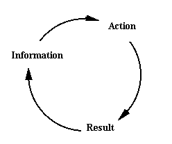
Figure 2: Closed-Loop view of the world
Behaviour which reinforces current systems performance is characteristic of positive feedback, a classic example of which is the process of accumulation of compound interest in a savings account. The influence diagram may be represented by a process such as that given by Figure 3:
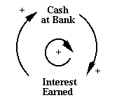
Figure 3: Positive Feedback Loop: Compound Interest
The process is that of a continually reinforcing process (note the + signs at the arrow-heads) and the loop is conventionally signed as a reinforcing loop with the positively signed arrow at its centre.
In contrast to the foregoing example of reinforcement, many real-life systems exhibit behaviour which constantly seeks to restore the system to its initial state or position, prior to the application of an external impetus. Take, for example, the operation of a simple thermostat to control a central-heating system. To control the system we might set the thermostat to some comfortable room temperature (say 20 degrees C) and settle down in a chair to read. As the outside air temperature falls below the desired thermostat setting a gap opens up between the desired temperature and the actual temperature in the room, so that the thermostat sends a signal to the boiler to fire. The boiler heats the water in the system, which is pumped to the radiators around the house. As the process continues, the radiators raise the temperature, thereby closing the gap between the actual and desired temperature which, when the gap reaches zero, signals the thermostat to switch off the boiler. This is a very simple, yet powerful means of controlling the level of heat in the home, and the process of negative feedback to a system is widely adopted in other control mechanisms. However, regardless of the context within which the control mechanism operates, the principle of negative feedback is identical in all cases. The process may be represented as follows: (Figure 4).
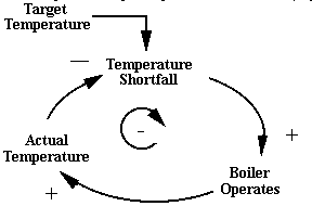
Figure 4: Negative, Balancing, Feedback Loop
A simple example of a negative feedback loop in macroeconomics is that which relates to the built-in stabilisers in the standard Keynesian macroeconomic model, having a Government and Trade sector. Such a model may be simply described as follows:
Y = C + I + G + (X -M) + (T - Tr) [1]
where Y = National Income, C = Consumption, I = Investment, X = Exports, M = Imports, T = Taxes, Tr = Transfer payments
Conventionally, the consumption function is denoted as a linear function of disposable income:
C = a + b(Y - T) [2]
where a = Autonomous Consumption, b = marginal propensity to consume, 0 < b < 1
Additionally, the import function is designated as
M = d + m(Y - T) [3]
where d = Autonomous level of Imports m = marginal propensity to import, 0 < m < 1 and the tax function as
T = e + tY [4]
where e = Autonomous taxation
t = marginal tax rate, again with 0 < t < 1.
Even with this very simple Keynesian model, which has exogenously-given Government expenditure, Transfer Payments, Investment and Exports, useful insights can be obtained whereby a decrease in taxation through a reduction in the marginal rate of income tax leads to an expansion in national income through the multiplier process, and into the degree to which the leakages from National Income operate to dampen or stabilise the extent to which National Income rises in response to the changes in the initial conditions of the model.
The simplest Keynesian model having no foreign sector, nor Government, posits
Y = C + I [5]
and C = a + bY yields the equilibrium level of National Income as: Y* = 1/(1-b) { a + I} [6]
where Y* denotes equilibrium Income level, and 1/(1-b) is the simple multiplier.
A unit change in the level of exogenous investment will therefore yield a change in National Income given by the value of the multiplier: 1/(1-b). More formally, it is the value of the partial derivative of National Income with respect to Investment. In the case of the more realistic, yet still simplified model represented by equations [1]-[4] the model may be solved for the equilibrium level of National Income:
Y* = 1/[1- (b + t - m)]{ I + X + G - Tr + a - d + e + (m - b)T}
and the corresponding principal multiplier values are given by the partial derivatives of National Income with respect to each of the exogenous variables.
The model indicates clearly that for values of b, t and m which are within the unit circle, the extent to which National Income rises in response to a change in the initial conditions is significantly attenuated in comparison with the simple model, due to the negative (compensating) mechanisms engendered within the leakage functions. These are characterised in some introductory macroeconomic texts as the "built-in stabilisers" of macroeconomic policy. Further debate on the performance of the model reduces to an empirical discussion on the relative magnitudes of m, b and t.
It is instructive to attempt to draw the influence diagrams operating within this process. Such influence diagrams can stimulate powerful learning by encouraging students to think about which variable influences others in processes, and in which direction, and the remarkable thing is that merely beginning to think in a qualitative way about dynamic processes can yield powerful insights into the important influences and variables to be considered. One especially powerful process is that of having students "talk their way through the loop", by articulating their thinking as they progress around the influence diagram. The technique, although extremely simple and consisting only of two basic types of feedback loop, is nonetheless extraordinarily powerful in its ability to map and represent complex processes. Building complexity and, possibly, more realism into the models, is simply a matter of adding additional loops. By this means it is possible to build models of great richness, which yield helpful insights into many processes, and which can provide predictions of system response to external changes in a variety of interesting ways, many of which are counter-intuitive to traditional ways of seeing the problem.
Although the causal loop diagramming technique described here is extremely powerful in obtaining qualitative insights into complex processes, it remains simply a qualitative exercise. A more useful approach should provide the practical means of extending these ideas into an operational process by building System Dynamics models capable of yielding quantitative results through simulation methods. STELLA, a software tool from High Performance Systems (High Performance Systems Inc., 45 Lyme Road, Hanover, New Hampshire, USA) is one of a small number of object-oriented modelling tools which seek to translate the ideas of Systems Thinking and System Dynamics directly into recognisable and operational models. The software provides a one-to-one correspondence between the ideas developed by Forrester et al and an executable model of systems behaviour, through the use of a small number of concepts and tools. These are shown in Figure 5.

Figure 5: STELLA Model Construction Tools
Flows, which use the visual metaphor of a pipe or conduit, allow for real resources to be transported around the model space. The "cloud" at the beginning of the flow icon represents an unrestricted source of resource, and that at the end represents a sink. The use of these metaphors allows for the system boundaries to be simply defined, although the software also permits more explicit definition of the system boundaries, by specifying and collecting together all resources, flows and links pertinent to a given sector within a sector boundary tool. Converters contain the algebraic relationships within a model, and act as scorekeeping variables. They may also be interpreted as functional relationships.
Connectors provide information links within a STELLA model, and may be thought of as analogous to conveying "electrical current" around a model, in contrast to the flow variable which conveys real resources.
The complete set of basic modelling tools is laid out along the top of the screen, as shown:
![]()
Figure 6: STELLA Basic Modelling Tools
By using this relatively simple set of tools, it is possible to model and simulate virtually any time-dependent process. The STELLA modelling environment offers a number of potential benefits, not the least being its completely generic nature. The brief discussion of Systems Thinking and System Dynamics given earlier neglected to mention that an astonishingly wide range of processes in a number of academic disciplines conform to a relatively small number of systems archetypes (Senge, 1990, Corben and Wolstenholme, 1994). In this respect, the modelling approach potentially offers significant intellectual economies of scale in representation of complex dynamic processes. A second potential benefit is provided by the visual modelling environment, in which much (if not, all) of the mathematics can be completely hidden from the student. As a STELLA model is constructed on computer screen, the software parses the logical structure of the model, not permitting an illegal connection according to the principles of information science and System Dynamics (Morecroft, 1994), and automatically generating the difference and differential equations describing system behaviour.
We illustrate this with reference to the extremely simple compound interest example used earlier to outline the positive feedback loop principle. The STELLA diagram shows the flow of Interest Earned into the accumulation of Cash on Deposit, which in turn feeds back into the quantity of Interest Earned. The STELLA diagram has an intuitive and logical interpretation which has been found to lend itself well to developing understanding in students\rquote own discussions of simple dynamic processes.
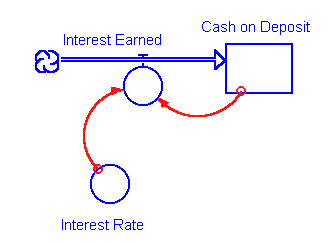
Figure 7: STELLA Representation of Interest Compounding Process
Cash_on_Deposit(t) = Cash_on_Deposit(t - dt) + (Interest_Earned) * dt

INIT Cash_on_Deposit = 100

INFLOWS: Interest_Earned = Cash_on_Deposit*Interest_Rate Interest_Rate = 0.08
STELLA provides a wide range of built-in functions (69 in all) for modelling financial, statistical and operational research processes, together with most of the usual spreadsheet functions. It is also possible to construct Boolean logic statements within converters and to specify one's own algebraic formulations.
Once the model is in a runnable state, as shown here, output from the process may be obtained through a variety of graphical and tabular devices, so that the numerical values generated from the model may be exported to spreadsheets, statistical packages and so on. This provides another potential benefit to modelling in economics, in that empirically obtained values of parameters may be entered directly into a constructed model and the results simulated very simply. An interesting example of this approach in the context of the optimal depletion rate of a fixed natural resource may be found in Ruth and Cleveland (1993).
A particularly powerful feature of the software is its ability to provide a range of sensitivity analyses on parameters. In the case of this simple model the only meaningful parameter to investigate is the rate of interest. Choosing the Sensitivity Analysis option brings up a dialogue box which offers selection of the parameter of interest. The default number of three "what-ifs" may be changed by the modeller, and the chosen values may be selected from user-specified Normal or Uniform Distributions, may be selected as ad hoc values, or if a start-value and end-value are chosen, the software will interpolate linearly in between these for successive sensitivity.
The STELLA package operates at three distinct levels. The Top level provides a High-Level Mapping capability within which one may lay out the overall logical structure of a model, and within which one may create a free-standing learning environment within which students may be encouraged to explore the logic and behaviour of the model, without altering its structure. This potentially offers a number of benefits in teaching, not least being that students may be prevented from destroying a given model. Once the behaviour of the model has been explored, and the results internalised, it may be appropriate to allow students to construct their own representations of economic processes, and to explore interactions between variables. Those who have adopted this "hands-on" approach to learning have claimed that significant benefits have accrued in individual and group learning as a consequence (Mandinach and Cline, 1990, 1994).
We give below, (see Appendix) a series of extremely simple model structures, of gradually increasing complexity, to show how widely this approach might be adopted in teaching and learning about fundamental economic principles. It must be understood that we are not seeking to replace conventional economic analysis by a process which has been received with some antagonism by the economics community in the past (Radzicki, 1988, 1990), but as a complement to existing approaches, and one which has potential for increased understanding of complexity, particularly dynamic complexity in the subject.
Economists who are interested in adopting this way of supplementing their existing resource materials by adopting the System Dynamics approach represented within the STELLA modelling environment may be interested to learn that the System Dynamics in Education Project at MIT (under the aegis of Jay Forrester, the founding father of Systems Thinking and System Dynamics approaches to modelling complexity) (Forrester, 1961, 1967, 1969, 1971a, 1971b) has recently put an information server on the Internet, containing a range of resources, models, templates and working models with documentation and examples of how the approach has been integrated into existing curricula. Details may be obtained via the Computers in Teaching I nitiative Centre for Economics at the University of Bristol (CTICCE@bristol.ac.uk). Others interested in developing learning materials in economics, finance, business management, and decision-making are encouraged to contact the author by e-mail (acboucher@eWorld.com).
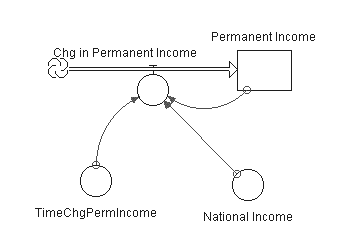
Simple Permaent Income Model
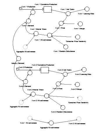
Radzicki's Duopoly Model