Visual identification of ARIMA models
Following Box and Jenkins (1970), ARIMA modelling has become a highly popular feature of time series analysis and a staple component of modules on forecasting, econometrics and statistics. Coverage of ARIMA modelling involves consideration of its constituent steps of identification, estimation, evaluation and forecasting. The focus of the present case study is on the first of these steps, namely the identification of ARIMA models. In particular, the present analysis centres on the visual identification of ‘pure’ ARIMA models for alternative data series via the use of autocorrelation functions (ACFs) and partial autocorrelation (PACF) functions.
It is well known that the visual identification of ARIMA specifications using ACFs and PACFs is not straightforward in many circumstances. In particular, the identification of mixed models (ARIMA specifications containing both an AR and an MA component) is problematic. However, while the visual identification of ‘pure’ processes (either AR or MA, but not both) might be more straightforward as a result of clear patterns within the theoretical ACFs and PACFs for alternative specifications, this itself is not without difficulty. The main issue that arises here is that the above properties relate to theoretical ACFs and PACFs rather than the sample or empirical functions observed in practice. As a consequence of this, findings might not be easy to interpret as, for example, observed patterns of decay may not provide an exact reflection of what is expected theoretically. The purpose of the present study is to provide empirical examples of the visual identification of alternative pure ARIMA models. As a consequence of the consideration of these specifications, the use of ACFs, PACFs, the Ljung-Box Q-statistic and the Akaike Information Criterion will be discussed and illustrated within the context of a practical setting.
To provide an example of the identification of a pure MA process, the variable y provided in the EViews file ARIMA_1.wf1 can be considered. Application of an Augmented Dickey-Fuller test to this series leads to overwhelming rejection of the unit root null hypothesis and hence the variable will be treated as stationary.[1] Plotting the ACF and PACF for this series with up to 20 lags considered, produces the following results:[2]

The Q-statistics clearly reject the null of randomness, or no structure, in every case considered with p-values of 0.000 observed. To identify this underlying structure, the ACF and PACF can be considered. The dashed lines accompanying the plotted values represent 5% critical values equal to ±2/√n which results in values of ±0.1 for the present example involving 400 observations. Considering the above findings, the ACF contains significant values at the first two lags, while the PACF exhibits decay in the form of an approximate damped sine wave. As a result, an ARIMA(0,0,2), or MA(2), model is suggested as an appropriate specification.
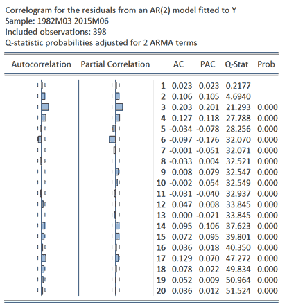
As a simple evaluation of the validity of the identified MA(2) specification, this model can be estimated and the properties of its residuals considered via an examination of their ACF and PACF, along with calculated Q-statistics. To provide a comparative examination of the properties of this model, analogous results can be considered for an alternative AR(2) model which acts a strawman against which the MA(2) specification can be compared. The results for both models are provided in the following tables. In contrast to the results for Y, inspection of the results for the residuals from the fitted MA(2) show no evidence of structure, with none of the AC or PAC values exceeding the 5% critical value and no Q-statistics rejecting their null of randomness. The results derived for the AR(2) model differ, with numerous significant AC and PAC values noted and all Q-statistics rejecting the null of no autocorrelation. Similarly, the calculated Akaike Information Criterion (AIC) values of 3.10 and 3.21 obtained for the MA(2) and AR(2) models, respectively, provide additional evidence of the former specification being preferred.

Identifying stationary pure processes: An ARIMA(p,0,0) process
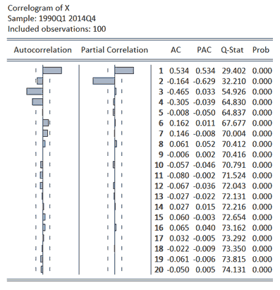
Following the above material which provides an example of the identification of an ARIMA(0,0,q) process, the EViews file ARIMA_2.wf1 offers the opportunity to consider the identification of an ARIMA(p,0,0), or AR(p), process. The ACF and PACF for the series x contained in the EViews file are reported below along with calculated Ljung-Box Q-statistics.[3] Considering the Q-statistics, the results provided clearly indicate the series has an underlying structure with p-values of 0.000 observed in all cases. To identify this underlying structure, the ACF and PACF can be considered. The dashed lines accompanying the plotted values represent 5% critical values which are equal to ±0.2 (= ±2/√n) in the present example involving 100 observations. The two significant values at the first two lags in the PACF and damped sine wave decay in the ACF suggest an ARIMA(2,0,0), or AR(2), as an appropriate specification.
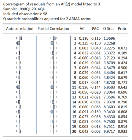
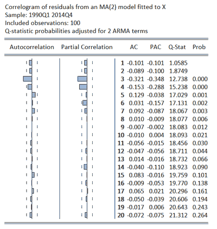
To provide a comparative analysis of the performance of the AR(2) specification, the properties of the residuals from this and those from an alternative ARIMA(0,0,2), or MA(2), specification can be considered. The results obtained from this analysis are presented below. The results show a clear preference for the AR(2) relative to the MA(2) specification with the former exhibiting no structure in its residuals via inspection of the ACF, PACF and Q-statistics. Similarly, calculated AIC statistics of 1.38 and 2.59 for the AR(2) and MA(2) models, respectively, demonstrate a preference for the former specification.
Summary
The above material has provided two empirical examples to allow consideration of the issue of ARIMA model identification. Recognising that identification can be less than straightforward in a variety of instances, the intention on this study has been to provide two clear examples to illustrate the identification of pure autoregressive and moving average models. In the process of doing so, illustrative material for the interpretation of autocorrelation and partial autocorrelation functions, Q-statistics and the Akaike Information Criterion has been provided.
References
Box, G. and Jenkins, G. (1970) Time Series Analysis: Forecasting and Control. San Francisco: Holden-Day. ISBN: 0816211043
Ljung, G. and Box, G. (1978) ‘On a measure of a lack of fit in time series models’, Biometrika, 65, 297–303. DOI: 10.1093/biomet/65.2.297 / JSTOR 2335207
[1] Including an intercept in the ADF testing equation and determining its order of augmentation via the AIC (Akaike Information Criterion) resulted in a test statistic of -6.22 with an accompanying p-value of 0.00.
[2] All results presented were obtained using EViews8.1.
[3] The variable x was considered a stationary process following application of an ADF unit root test in the manner employed above for y.