Volume 12, Issue 2, 1998
The use of “pick-up” matrices to produce separate quarterly series from an annual series
- Guy Judge
CALECO Research Group
University of Portsmouth
Introduction
Most government statistical agencies provide information in electronic form for many seasonally observed (e.g. quarterly or monthly) macroeconomic time series. For example in the UK you can download such information from the Office for National Statistics Time Series databank at the MIDAS site at Manchester University http://midas.ac.uk/ Such series will generally be delivered as one continuous series (a single vector). However you may wish to separate the series into 4 (or 12) series each of which contains only the values relevant for that particular quarter (or month). This might be simply because you want to plot each series separately, or because you intend to use a model which treats observations from each season differently (e.g. the Periodic Autoregression Model - see Franses (1995), (1996)).
There are various ways such series can be separated. Of course the simplest and most basic approach is “by hand” where you manually run down the series copying each relevant element to a position in one of the new quarterly series. If the data are in a spreadsheet this operation could be undertaken by copying the cell contents, moving to the next relevant element and repeating.
If the series is a long one, or if the process needs to be repeated for many such series, it may occur to you to write a spreadsheet macro to copy the element, skip the next three (eleven) elements, copy again etc.. A similar approach could be taken using other programming languages or tools.
However there is an alternative procedure based on premultiplying the vector by a suitably designed matrix (which I refer to as the “pick-up” matrix) which can achieve the desired effect in a single step.
The “pick-up” matrix method
To explain the method let us work with a concrete example.

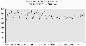
Figure 1 Real Consumers’ Expenditure on Beer in the UK: 1986Q1-1997Q4
Click above to download image
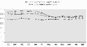
Figure 1 shows a time series plot of the quarterly series CCBNQU (for the period 1986Q1 to 1997Q4) which was downloaded from the MIDAS site. The series is Consumers’ Expenditure on Beer in £million at constant (1990) prices and it has not been seasonally adjusted. Indeed the time series plot shows clearly that seasonality is important for this series, although after 1992 not only does the level of the series appear to have dropped quite markedly, but also the seasonal pattern seems to have changed. To get another view of these changes it can be helpful to plot each quarter as a separate series as in Figure 2.

Figure 2 Real Consumers’ Expenditure on Beer in the UK plotted as
four separate quarterly series
Click above to download image
Here you can see that the values in each quarter fell dramatically in the early nineties, recovering slightly recently. However the seasonal pattern has changed with quarter 4 being overtaken by the quarter 2 and quarter 3 values. It is not the purpose of this paper to explain these patterns (although part of the explanation may be the fact that large quantities of beer are now imported directly by consumers from continental Europe). Instead we wish to describe a simple method for breaking up the original series into four separate quarterly series.
Our series consists of 12 years of quarterly observations. If we store the values in a single column vector y it will be of the order 48x1. What we want are 4 separate 12x1 column vectors y1, y2, y3 and y4, each containing the observations pertaining to the relevant quarter.
To obtain y1 from y we must premultiply y by a 12x48 matrix called say P1 which is designed to pick up only the first quarter observations. The first row of P1 will have a 1 as the first element and zeros elsewhere. The second row will have a 1 as the fifth element and zeros elsewhere. Each row will have just a single element which is equal to one - to pick up the desired element from y - with all the other values equal to zero.
Formally for i=1 to 12, j=1 to 48 pij= 1 when j = 4(i-1) + 1, 0 otherwise.
Similar matrices P2, P3 and P4 can be defined to pick up the quarterly series y2, y3 and y 4.
For P2 for i=1 to 12, j=1to 48 pij= 1 when j = 4(i-1) + 2, 0 otherwise,
for P3 for i=1 to 12, j=1to 48 pij= 1 when j = 4(i-1) + 3, 0 otherwise,
and for P4 for i=1 to 12, j=1to 48 pij= 1 when j = 4(i-1) + 4, 0 otherwise.
Hint: If you plan to do this on a spreadsheet the quickest way to create the P matrices is to fill up the block with zeros and then replace the elements which need to be 1.
The method can of course be modifed for monthly series. In general if there are S seasons (s=1,2,...S) and N years (i=1,2,...N) giving n =NS observations in the original series we define pick-up matrices Pk, k=1,2,...S such that pij= 1 when j = S(i-1) + k, 0 otherwise.
Differencing, summation and other filters.
A similar approach to that outlined above can be used to obtain series which are differenced, summed or (linearly) filtered in some other way.
For example the nx1 vector y containing the observations of a variable can be premultiplied by the (n-1)xn matrix D1, where dij= 1 for j=i, -1 for j =i+1, 0 otherwise, to obtain the (n-1)x1 vector of first differences.
The filter (1-B4) could be applied by premultiplying y by the (n-4)´n matrix D4 which has dij = 1 for j=4(i-1)+1, -1 for j =4(I-1)+4, 0 otherwise, to give a vector of yt-yt-4 values.
The seasonal sum filter 1+B+B2+B3 could be obtained by premultiplying y by S4 where sij= 1 for i=j, i=j+1, i = j+2, i =j+3, 0 otherwise.
Other factors of 1-B4 such as (1-B2) which are required in the HEGY test for seasonal unit roots could be created in the same way (see Hyllberg et al.(1990)).
While it might be argued that these filters could perhaps be most easily applied using tools within the chosen regression software package, there may be occasions when one wants to separate the different seasonal series after differencing (e.g. if one wanted to plot not the levels of the four quarterly series but their rates of growth). In this case you would apply the D1 filter first and then the pickup matrices P1 to P4. It might be convenient to do all this preparatory work within the spreadsheet environment before you run the regression software.
References
Franses, P H (1995)
A Vector of
Quarters Representation for Bivariate
Series. Econometric Reviews. Volume 14 No 1 pp 55-63
Franses P H (1996)
Periodicity and Stochastic Trends in Economic Time
Series. Oxford University Press.
Hyllberg S et al. (1990)
Seasonal Integration and Cointegration. Journal
of Econometrics Vol 44 pp 215-238.

