

The development and use of optimisation models is well established. However, the use of many models has been restricted in some fields of economic analysis where the problem is large in size and there are a large number of non-linear interactions. In most cases, the use of linear approximations or simplification of the model has been necessary in order to derive a solution.
Genetic algorithms (GA) are an evolutionary optimisation approach which are an alternative to traditional optimisation methods. GA are most appropriate for complex non-linear models where location of the global optimum is a difficult task. It may be possible to use GA techniques to consider problems which may not be modelled as accurately using other approaches. Therefore, GA appears to be a potentially useful approach.
GA follows the concept of solution evolution by stochastically developing generations of solution populations using a given fitness statistic (for example, the objective function in mathematical programmes). They are particularly applicable to problems which are large, non-linear and possibly discrete in nature, features that traditionally add to the degree of complexity of solution. Due to the probabilistic development of the solution, GA do not guarantee optimality even when it may be reached. However, they are likely to be close to the global optimum. This probabilistic nature of the solution is also the reason they are not contained by local optima.
The list of topics to which genetic algorithms have been applied is extensive. These include scheduling, time-tabling, the travelling salesman problem, portfolio selection, agriculture, fisheries etc. In this paper the basic features, advantages and disadvantages of the use of GA are discussed. A brief review of GA software is given. A small nonlinear fisheries bioeconomic model is used to compare the GA approach with a traditional solution method in order to measure their relative effectiveness. General observations of the use of GA in nonlinear programming models are also considered.
The conceptualisation of GA in current form is generally attributed to Holland, 1975. However, particularly in the last ten years, substantial research effort has been applied to the investigation and development of genetic algorithms. Goldberg, 1989 gives an excellent introductory discussion on GA, as well as some more advanced topics.
Genetic algorithms are a probabilistic search approach which are founded on the ideas of evolutionary processes. The GA procedure is based on the Darwinian principle of survival of the fittest. An initial population is created containing a predefined number of individuals (or solutions), each represented by a genetic string (incorporating the variable information). Each individual has an associated fitness measure, typically representing an objective value. The concept that fittest (or best) individuals in a population will produce fitter offspring is then implemented in order to reproduce the next population. Selected individuals are chosen for reproduction (or crossover) at each generation, with an appropriate mutation factor to randomly modify the genes of an individual, in order to develop the new population. The result is another set of individuals based on the original subjects leading to subsequent populations with better (min. or max.) individual fitness. Therefore, the algorithm identifies the individuals with the optimising fitness values, and those with lower fitness will naturally get discarded from the population.
Ultimately this search procedure finds a set of variables that optimises the fitness of an individual and/or of the whole population. As a result, the GA technique has advantages over traditional non-linear solution techniques that cannot always achieve an optimal solution. A simplified comparison of the GA and the traditional solution techniques is illustrated in Figure 1. Non-linear programming solvers generally use some form of gradient search technique to move along the steepest gradient until the highest point (maximisation) is reached. In the case of linear programming, a global optimum will always be attained (). However, non-linear programming models may be subject to problems of convergence to local optima, or in some cases, may be unable to find a feasible solution. This largely depends on the starting point of the solver. A starting point outside the feasible region may result in no feasible solution being found, even though feasible solutions may exist. Other starting points may lead to an optimal solution, but it is not possible to determine if it is a local or global optimum. Hence, the modeller can never be sure that the optimal solution produced using the model is the “true” optimum.
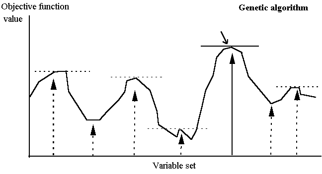

Figure 1(a/b). Comparison of gradient search technique and genetic
algorithm approach.
Click above to download the images
For the genetic algorithm, the population encompasses a range of possible outcomes. Solutions are identified purely on a fitness level, and therefore local optima are not distinguished from other equally fit individuals. Those solutions closer to the global optimum will thus have higher fitness values. Successive generations improve the fitness of individuals in the population until the optimisation convergence criterion is met. Due to this probabilistic nature GA tends to the global optimum, however for the same reasons GA models cannot guarantee finding the optimal solution.
The GA consists of four main stages: evaluation, selection, crossover and mutation. The evaluation procedure measures the fitness of each individual solution in the population and assigns it a relative value based on the defining optimisation (or search) criteria. Typically in a non-linear programming scenario, this measure will reflect the objective value of the given model. The selection procedure randomly selects individuals of the current population for development of the next generation. Various alternative methods(2) have been proposed but all follow the idea that the fittest have a greater chance of survival. The crossover procedure takes two selected individuals and combines them about a crossover point thereby creating two new individuals. Simple (asexual) reproduction can also occur which replicates a single individual into the new population. The mutation procedure randomly modifies the genes of an individual subject to a small mutation factor, introducing further randomness into the population.
This iterative process continues until one of the possible termination criteria is met: if a known optimal or acceptable solution level is attained; or if a maximum number of generations have been performed; or if a given number of generations without fitness improvement occur. Generally, the last of these criteria applies as convergence slows to the optimal solution.
Population size selection is probably the most important parameter, reflecting the size and complexity of the problem. However, the trade-off between extra computational effort with respect to increased population size is a problem specific decision to be ascertained by the modeller, as doubling the population size will approximately double the solution time for the same number of generations. Other parameters include the maximum number of generations to be performed, a crossover probability, a mutation probability, a selection method and possibly an elitist strategy, where the best is retained in the next generation’s population.
Unlike traditional optimisation methods, GA is better at handling integer variables than continuous variables. This is due to the inherent granularity of variable gene strings within the GA model structure. Typically, a variable is implemented with a range of possible values with a binary string indicating the number of such values; i.e. if x1Î[0,15] and the gene string is 4 characters (e.g. “1010”) then there are 16 possibilities for the search to consider. To model this as a continuous variable increases the number of possible values significantly. Similarly, other variable information which aids the search considerably are upper and lower bound values. These factors can affect convergence of the model solutions greatly.
An excellent starting place for information is The Genetic Algorithms Archive(3). It contains many links to public domain software, to research conducted by leading experts in the field and other useful pointers.
Until recently the majority of GA software used was primarily available in the public domain or developed by users specifically for a problem. However, with increased computer power and further GA enhancements which have been proposed, more commercial systems are becoming available. One of the leading commercial software packages devoted to GA is the Microsoft Excel add-in EVOLVER (currently version 4) - see Pascoe, 1996 for a review of EVOLVER V3 compared to a traditional nonlinear programming optimiser. The significant advantage of such a package is the familiar, user-friendly interface which the developers claim requires no knowledge of computer programming or GA theory to use. However, in a similar way to using SOLVER for linear programming, users who know little about the encompassing subject area will often produce badly structured models.
One of the first publicly available systems was GENESIS (Grefenstette, 1984) which has since been used as the building block for many other GA systems, such as GENEsYs (Baeck, 1992). The majority of existing GA tools are written in C/C++. Many are available free for non-commercial activity. The modeller typically implements the model directly into the code of the computer program. Generally, the only requirement of a fitness function is to return a value indicating the quality of the individual solution under evaluation. This gives the modeller almost unlimited freedom in building the model, therefore a diverse range of modelling structures can be incorporated into the GA. Although, C/C++ is a robust programming language for algorithmic software development, this adds to the expertise required by the modeller. Typically, a user-friendly interface is not available as this is not intrinsic to the GA search process. This is definitely a disadvantage over the usability and history of development of traditional optimisation modelling approaches, especially in mathematical programming.
Although GA systems follow the same general algorithmic procedure, each GA system is designed and implemented in a slightly different way, using alternative random number generators and various compilers. Therefore no two systems will optimise a model using exactly the same path. Other differences which have a significant effect on the solution process are the various parameter options which are implemented in each solver - for example some of the key parameters are the selection method, crossover rate, mutation rate, recombination scheme, elitist strategy and population size. SGA, as described by Goldberg, 1989, has one selection method and one recombination scheme implemented whereas a more developed system such as GENEsYs has seven selection methods, four recombination schemes and even two alternative mutation procedures.
GA are particularly applicable to unconstrained (or largely feasible) problems as the individual solutions of a population are then directly comparable in terms of their fitness. In this case, where feasibility is assured, the search method has no difficulties in measuring the quality of solution with respect to infeasibility (see the following example). A number of alternatives have been proposed for the handling of constraints; e.g. infeasible solution rejection, penalty functions, maintain feasibility using specialised operators, and repair the infeasible individual. Penalty functions are the most commonly applied technique. Compared to nonlinear programming models, less “active” variables and constraints are necessary in the model, i.e. many variables may be dependent on others often described by the constraints, and therefore explicit definition as control variables may not be necessary (see the following example). Convergence slows significantly for constrained problems where infeasibility is a factor. However, GENOCOP3 (Michalewicz, 1996) incorporates methods to enable internal management of nonlinear constraints, i.e. once obtained feasibility is maintained through specialised operators.
A simple fisheries bioeconomic model is discussed below, where 3 classes of boat (i) catch 3 species of fish (j) in a given region. An optimal allocation of the resource is sought which maximises economic profit. Table 1 shows the data definitions. There are 5 variable classes (15 variables) in the nonlinear programme; i.e. boats (xb) and effort (xe) of boat class i, and catch (xc), landings (xl) and fishing mortality (xf) of species j. This problem is solved with the selected genetic algorithm solvers as well as a traditional nonlinear programming solver in order to compare the relative merits of the approaches. Both the continuous and integer forms of the model are considered, as strictly xb (number of boats) is an integer variable set. This problem also demonstrates the flexibility of GA and the type of models which can be considered.
Table 1: Model data.
|
Variable |
Description |
Values |
|||||||||
|
Pj |
Price of fish species j |
{2.5, 2, 1.5} |
|||||||||
|
Fi |
Fixed Costs of boat class i |
{1, 0.8, 0.8} |
|||||||||
|
Vi |
Variable Costs of boat class i |
{0.01, 0.008, 0.008} |
|||||||||
|
Qij |
Catchability coefficient of fish species j by boat class i |
|
|||||||||
|
Kj |
Carrying capacity of fish species j |
{2000, 2500, 4000} |
|||||||||
|
Rj |
Growth rate of fish species j |
{0.1, 0.5, 0.3} |
The mathematical description of the nonlinear programme, with both a nonlinear objective function and nonlinear constraints, is given below;
 (1)
(1)
subject to,
 (2)
(2)
 (3)
(3)
xlj £ xcj ( j =1,...,3) (4)
xb, xe, xf, xc, xl ³ 0 (5)
where the objective function (1) denotes the economic profit for the fishery which is determined by revenue from landings minus the associated fixed and variable costs of the fishing. Equation (2) defines the fishing mortality, equation (3) then evaluates catch from this fishing mortality rate and equation (4) constrains landings to be no greater than catch. The (control) variables xb, xe and xl have upper bound values of {100, 100, 100}, {275, 160, 200} and {500, 500, 500} respectively.
By inspection, it is clear in the nonlinear programming problem above that xf are dependent variables, i.e. their value is dependent on the values of xe and xb. In turn xc is dependent on xf. It follows in the fitness function of the GA that these dependent variables can be simply calculated from the probabilistic (or control) variables xe and xb. A simple repair approach is implemented for equation (4) in the fitness function, where if the constraint is violated then xl* is reset equal to the relevant xc*. Therefore, when the constrained NLP model is built in the GA it can be interpreted as an unconstrained 9 variable model(4) where the returned fitness value is the NLP objective function value of economic profit (r).
The NLP model was solved in GAMS (Brooke, Kendrick and Meerhaus, 1988) using the CONOPT solver which in the version used was not capable of solving a model with integer restrictions. Consequently, an approximating approach was used by rounding each variable to its nearest integer value for the integer solution. Four public domain GA systems were selected for comparison; GENEsYs (Baeck, 1992), GENOCOP3 (Michalewicz, 1996), FORTGA(5) (Carroll, 1997) and multi-variable SGA(6) (Goldberg, 1989). A population size of 70 and an elitist strategy was used for each (except SGA which was restricted to a population size of 30), however other parameters were chosen based on several runs of the model. Table 2 shows the results from the model with continuous variables and table 3 shows the results with the boat variables having integer restrictions. All optimisations were performed on a Pentium 200Mhz PC compatible computer.
Table 2: Continuous Solutions.
|
Profit |
Boats - xb |
Effort (h) - xe |
Time† |
|
1 |
2 |
3 |
1 |
2 |
3 |
(secs) |
||
|
GAMS |
1176.458 |
0.90 |
6.96 |
2.32 |
275 |
160 |
200 |
0.3 |
|
GENESYS |
1176.458 |
0.90 |
6.96 |
2.32 |
275 |
160 |
200 |
76 |
|
GENOCOP3 |
1176.458 |
0.90 |
6.96 |
2.32 |
275 |
160 |
200 |
19 |
|
FORTGA |
1176.444 |
0.90 |
6.95 |
2.34 |
275 |
160 |
199.22 |
268 |
|
SGA |
1176.441 |
0.90 |
6.93 |
2.34 |
275 |
160 |
199.56 |
885 |
Table 3: Integer Solutions.
|
Profit |
Boats - xb |
Effort (h) - xe |
Time† |
|
1 |
2 |
3 |
1 |
2 |
3 |
(secs) |
||
|
GAMS |
1171.698 |
1 |
7 |
2 |
275 |
160 |
200 |
* |
|
GENESYS |
1175.799 |
1 |
7 |
3 |
248.25 |
159.77 |
155.14 |
22 |
|
GENOCOP3 |
1175.799 |
1 |
7 |
3 |
248.40 |
159.73 |
155.21 |
14 |
|
FORTGA |
1175.799 |
1 |
7 |
3 |
248.14 |
159.77 |
155.14 |
67 |
|
SGA |
1175.797 |
1 |
7 |
3 |
249.22 |
159.69 |
155.18 |
288 |
* - This was an approximated solution from the continuous solution.
† - Time in CPU seconds until best solution.
In all the genetic algorithms implemented (tables 2 and 3), convergence to the optimal solution for the model is very close to full achievement. It is clear in these results that simply approximating an integer solution to the model from the optimal continuous solution does not give the optimal integer solution. As expected, it is also noticeable that the GA with integer restrictions achieves the optimal solution far quicker than the continuous cases. The differences in solution times between the GA solvers (for exactly the same model structure) is significant. This highlights the point that different GA implementations are more advanced and may be more suitable for some model types than others. Also, parameter options and values have a significant effect.
It should be noted that for the GAMS model, a starting point of the origin (i.e. all variables zero) is reported to be locally optimal thus stopping optimisation. The solver advises at this point to use a better starting solution. Any non-zero initial solution for xb and xe is satisfactory.
Figure 1 shows the typical convergence rates between two selection strategies (i.e. tournament selection and roulette wheel selection) in FORTGA for the integer case. Three runs were performed with each selection method over 10,000 generations and the best run plotted in figure 1. In all runs the tournament selection performed best, achieving the best solution of 1176.444. Roulette wheel selection was not as successful, converging to a best value of 1170.760 in the 10,000 generations completed. For this model, it appears that the convergence is generally slower using the roulette wheel selection than tournament selection.
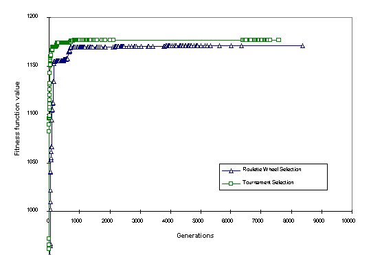
Fig 3. Typical progress with two alternative selection methods
(FORTGA continuous)
Click above to download image
In the genetic algorithms, a maximum generation count was used as the stopping criteria, and determined by performing a number of optimisations until a satisfactory level was ascertained. Other parameters were also evaluated through a number of trial runs, although default parameter values were preferred where possible.
It is a typical occurrence in modelling real-life problems that approximations are made in order to accommodate the capability of the solver. This is due to the natural size and complexity of models, where many of the variable interactions form non-linear relationships in the model. Where solution is not possible by traditional approaches, GA may be able to offer a viable alternative. As in the example above, it would not be expected for a constrained mathematical programming problem to be solved faster by GA, which is a probabilistic search method, than by a traditional optimisation approach, which is a guided search method and has been developed and successfully applied to many models of this type over the years. Genetic algorithms should not be regarded as a replacement for other existing approaches, but as another optimisation approach which the modeller can use.
The main advantage of GA is that models which cannot be developed using other solution methods without some form of approximation can be considered in an unapproximated form. Size of the model, i.e. number of probabilistic variables, has a significant effect on the speed of solution therefore model specification can be crucial. Unlike other solution methods, integer variables are easier to accommodate in GA than continuous variables. This is due to the resulting restricted search space. Further, variable bound values can be applied to achieve similar results.
There are a number of factors which must be taken into consideration when developing a genetic algorithm model; there are typically many standard parameters which can be modified to affect the performance of the optimisation (see section 2), variable specification (probabilistic or deterministic), tight variable bounds, weighting strategies and constraints. Unconstrained problems are particularly suitable for consideration as constraints require the management of possible infeasibility, which may slow down the optimisation process considerably. Generally, a standard genetic algorithm is taken for specific development of the problem under investigation where the modeller should take advantage of model structure for effective implementation.
The ease of implementation of a model within a GA is directly related to the knowledge of the modeller on three topics; programming (e.g. C/C++, FORTRAN, PASCAL etc.), model understanding and basic knowledge of GA. It is beneficial spending time to construct an efficient model with (few) control variables in a largely feasible variable space. Instruction guides and manuals of freely available software do not generally cover every aspect of the system being used, but offer an introduction to the environment along with brief reference topics. Differences between GA software codes concerning model development and model optimisation are very small. Parameters are usually either communicated to the program through (a combination of) the command-line, parameter file and directly in the code.
Constraints are difficult to incorporate into a GA, as generally it is left to the fitness function to manage and quantify possible infeasibility. For problems where a large feasible set of solutions exist, constraints do not pose the same problem as for a small feasible set. This is because the fitness function must generally determine the level of infeasibility and optimality as one fitness statistic. If feasible solutions are easily determined, then fitness is easily described.
It is difficult to generalise on which is the “best” genetic algorithm to use for a given problem, however the more advanced and highly developed GA solvers will generally offer faster convergence leading to a more accurate solution. Such GA are significantly more complex than a basic GA (e.g. SGA), and will typically be used as a ‘black-box’.
As models have become increasingly more detailed, the types of questions which managers hope to find answers to have also become more complex. New techniques can expand the range and relevance of models in solving real-world issues. Such a tool will both contribute to the methodological development of modelling as well as having immediate practical benefits in terms of increasing the range of management questions that can be addressed by such models.
[Baeck, 1998]
Baeck, T. A User’s Guide to GENEsYs 1.0 , Department of
Computer Science, University of Dortmund, 1992.
[Brooke, 1998]
Brooke, A.D., D. Kendrick and A. Meerhaus, GAMS: A User’s Guide,
Scientific Press, 1988.
[Carroll, 1997]
Carroll, D.L., Fortran GA - Genetic Algorithm Driver V1.6.4, Users
Guide, 1997.
[Goldberg, 1989]
Goldberg, D.E., Genetic Algorithms in Search, Optimization, and
Machine Learning, Addison-Wesley, USA, 1989.
[Grefenstette, 1984]
Grefenstette, J.J., GENESIS: a system for using genetic search procedures,
Proceedings of the 1984 Conference on Intelligent Systems and Machines,
161-165, 1984.
[Holland, 1975]
Holland, J.H., Adaptation in Natural and Artificial Systems,
University of Michigan Press, USA, 1975.
[Michalewicz, 1996]
Michalewicz, Z., Genetic Algorithms + Data Structures = Evolution
Programs, 3rd ed., Springer, 1996.
[Pascoe, 1996]
Pascoe, S., A tale of two solvers: Evolver 3.0 and GAMS 2.25, The
Economic Journal, 106(1), 264-271, 1996.