Volume 9, Issue 2, 1995

Examples for Economists with DERIVE 3.0: Long- and Short-run Costs
Barry MurphyUniversity of Portsmouth
The relations between long- and short-run average, marginal and total costs have been a standard topic in elementary economics since Viner's (1931) account. As is well known, Viner's original account contains an error which his draughtsman Y. K. Wong attempted unsuccessfully to prevent. Viner (1950) corrects this error, which relates to the property that the long-run average cost is the lower envelope of the family of short-run average cost curves.
The purpose of this note is to use DERIVE 3 to illustrate the whole topic for an arbitrary well-behaved technology. In particular, we can use DERIVE to illustrate a point that is not usually brought out in elementary accounts. There is a much more specific relation between long-run and short-run average and total cost curves beyond the property noted above. In particular, the functional form of short-run cost is intimately related to the functional form of long-run cost.
Details of the DERIVE file used are given in the appendix. It is short enough to be typed directly. It can be used even by an inexperienced DERIVE user. Two principal functions are defined.
STC(tc,w,r,y,k) simplifies to the short-run total cost function corresponding to the long-run total cost function tc. tc depends on the price of variable input w, the price of fixed input r, and output y. The symbol for short-run fixed input is k.
TC(stc,w,r,y,k) simplifies to the long-run total cost function corresponding to the short-run total cost function stc. stc depends on the price of variable input w, the level of fixed input k and output y. The symbol for the price of the short-run fixed input is r.
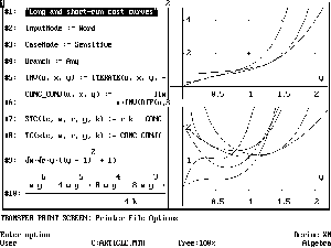
These functions are mutual inverses. Applying STC to a well-behaved long-run total cost function, and then applying TC to the result gives one back the original long-run total cost function. Similarly, applying TC to a well-behaved short-run total cost function and then applying STC to the result gives one back the original short-run total cost function. The arguments of TC and STC are dummy variables, and can be chosen by the user. Once the short- and long-run total cost functions corresponding to a particular technology are obtained using STC and LTC, the average and marginal functions can be obtained and plotted using DERIVE. Figure 1 shows an example for the long-run total cost function given in expression #9, which corresponds to a Cobb-Douglas technology with variable returns to scale. This is a TIF file screen capture produced by DERIVE itself. A 16-colour image is available in the on-line version of this Review. McFadden (1978) specifies what well-behaved means in this context. Informally, this is easily explained.
tc and stc must be non-negative functions of the non-negative variables (w, r, y, k).
tc must be concave and homogeneous of degree 1 (w, r), and increasing in (w, r) for positive y.
tc must be increasing in y, for strictly positive (w, r).
stc - rk must be concave and homogeneous of degree 1 in w, i.e. proportional to w.
stc - rk must be increasing in y for strictly positive w.
stc - rk must be decreasing and convex in k when stc is strictly positive.
In addition tc and stc must satisfy a regularity condition: it is sufficient if both are continuous. stc - rk is known as the restricted cost function by certain authors (e.g. Gorman (1976) and Varian (1994)). Others reserve the term for stc itself (e.g. Deaton and Muellbauer (1980)).
This DERIVE application depends on solving for r in the equation tc/ k = r and for k in the equation stc/ r = k, so we assume also that these solutions exist and are unique, and that DERIVE can find them.

Figure 1 Long- and short-run cost curves for tc = expression #9 (w = r = 1, k = 1/4, 3/4).
- a marginal cost curve cuts the corresponding average cost at the
point of minimum average cost
- an average curve is increasing (resp. decreasing) when the
corresponding marginal curve is above (resp. below) it
- the minimum point of a marginal curve is at the same output as
a point of inflection of the corresponding total curve
- the long-run average (resp. total) cost curve is the lower
envelope of the family of short-run average (resp. total) cost
curves
- long-and short-run total cost curves are tangent at the output at which the long- and short-run average cost curves are tangent, and at which long-and short-run marginal cost intersect.
Figure 1 contains a possible surprise for a student: in this case the short-run marginal cost curves are not U-shaped.

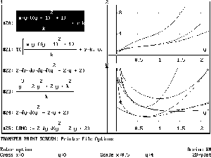
Figure 2 Long- and short-run cost curves for stc = expression #20 (w = r = 1, k = 1/4,3/4).
A subsidiary purpose of this note is to illustrate the use of DERIVE and similar software in producing diagrams to illustrate points of quantitative economics. Too often, even excellent text-books are filled with art-work that throws little light on interesting features of a model or its dependence on underlying parameters. Such pictures may be too perfect in appearance or symmetry, or merely uninformative on points of importance such as limiting slopes. A good example of this is the Giffen good diagram which every student of economics learns. The phenomenon is next to impossible in practice, and the usual picture throws little light on why this is so. By contrast, a diagram may be less showy than art-work, but it can provide accurate information on the model being presented and enable its dependence on model parameters to be assessed.
It should be emphasised that this DERIVE application will work with any well-behave cost functions for which DERIVE can solve the equations mentioned above, and not merely for the examples illustrated here.
Appendix Users of the DERIVE procedures outlined above do not need to know any of the following details. They are provided in case comments, improvements or suggestions are forthcoming.
The DERIVE file (an ASCII file) CC.MTH consists of the following lines of text:
"CC.MTH: a file for (concave) conjugacy with respect to one real variable"
" © Barry Murphy, University of Portsmouth, May 1995" InputMode:=Word
CaseMode:=Sensitive
Branch:=Any
"It may help to restrict variable domains appropriately"
"This solves u(x)=y for x (if it can)"
INV(u,x,y):=ITERATE(u,x,y,-1)
"This is the (concave) conjugate of the (concave) function u(x)"
CONC_CONJ(u,x,y):=LIM(x*y-u,x,INV(DIF(u,x),x,y))
"You need to check the answer; see R. Tyrrell Rockafellar, Convex Analysis"
"Application: short and long-run cost functions"
STC(tc,w,r,y,k):=r*k-CONC_CONJ(tc,r,k)
TC(stc,w,r,y,k):=CONC_CONJ(-(stc-r*k),k,r)
"Example: these two show that TC and STC are mutual inverses"
SQRT(w)*SQRT(r)*y*((y-1)^2+1)
(w*y^6-4*w*y^5+8*w*y^4-8*w*y^3+4*w*y^2+4*k^2*r)/(4*k)
Only the seven lines in bold type are essential, and these should be typed exactly as above, each line after issuing the Author command in DERIVE. The remaining lines are inessential, consisting of comments or examples. The first three lines in bold type specify that case-sensitive word input is to be used, and that the simplest branch of the solutions to an extended rational equation be used.
The file depends on the idea of concave conjugacy explained, for example, in Rockafellar (1970). The concave conjugate of the concave function u is defined by u*(y) = inf x {x y - u(x)} By contrast, the convex conjugate of the convex function v is defined by v*(y) = sup x {x y - v(x)}
 Since v = -u is
convex if u is concave, in that case we have u*(y) = -v*(-y). The
file CC.MTH obtains the concave conjugate of u by solving the
equation y = du(x)/dx for x and then substituting into xy - u(x).
If u is concave and differentiable this condition is necessary
and sufficient for the infimum in the definition to be attained
at an interior point of the domain of u. In practice, the DERIVE
solution has to be checked: the first-order condition may be
attained even if u is not concave (e.g. if convex).
The defined function INV solves y = u(x) for x if it can: INV(LN(x),x,y)) simplifies to EXP(y) and INV(x^a,x,a)) simplifies to y^(1/a). The defined function CONC_CONJ substitutes the solution for x from y = du(x)/dx into xy - u(x). DERIVE's way of doing this is by taking a limit.
The defined functions STC and TC expresses two ideas. The short-run total variable cost function is the level of fixed cost plus the negative of the concave conjugate of the long-run total cost function, and the long-run total cost function is the concave conjugate of the short-run total variable cost function. The operation of conjugacy is of more general interest in economics, and it would be of value to be able to calculate the conjugate of a function of several variables. This requires the solution of the multivariate equivalent of the equations tc/ k = r and stc/ r = k.
Unfortunately, my experiments suggest that this is too difficult for DERIVE except in special cases.
References
- Boulding, K. E. and G. J. Stigler, Readings in Price Theory, George Allen and Unwin Ltd, 1953.
- Deaton, A. S. and J. Muellbauer, Economics and Consumer Behaviour, Cambridge University Press, (1980).
- Gorman, W. M. "Tricks with utility functions", in Artis, M. and A. R. Nobay (eds.), Essays in Economic Analysis, Cambridge University Press (1976).
- McFadden, D., "Cost, Revenue, and Profit Functions", in McFadden, D, and M. Fuss (eds.), Production Economics: A Dual Approach to Theory and Applications, Volume 1, pp. 3-109, North-Holland, 1978.
- Rockafellar, R. T., Convex Analysis, Princeton University Press, 1970.
- Varian, H. R., Microeconomic Analysis, third edition, W. W. Norton & Co. Inc., 1994.
- Viner, J., "Cost Curves and Supply Curves", Zeitschrift fur National Ekonomie, Volume III, pp. 23-46, reprinted in Boulding and Stigler (1953), pp. 198-226, 1931.
- Viner, J., "Supplementary Note", in Readings in Economic Analysis, R. V. Clemence (ed.), Addison-Wesley Press, 1950, reprinted in Boulding and Stigler (1953), pp. 227-232, 1950.
This is the first of a series of articles on DERIVE use in economics. Comments and contributions are welcome. The on-line version of this Review contains Figure 1 and Figure 2 above as 16-colour graphics files (not yet available! Webmaster...). They are worth a look. I will provide a copy of the file CC.MTH and of the DERIVE files used to construct the Figures to any interested reader.

