

This paper shows how spreadsheet simulations can be used to teach the Taylor-Romer model of macroeconomic stabilisation policy. This model is both a simpler and more realistic description of the modern implementation of monetary policy than the traditional IS-LM-AS model. The simulation exercises are quite appropriate at the introductory (or principles) level. One modification is proposed to the model; that is, the replacement of the level of output by the growth rate of output. This allows for a direct illustration of the short run trade-off between growth and inflation in the model.
Cahill and Kosicki (2001) have shown in this journal how spreadsheet simulations can be used to demonstrate the IS-LM-AS model of short run macroeconomic fluctuations. This model has been an effective workhorse for 30 years and remains useful for modelling the adjustment path to some shocks as Cahill and Kosicki (2001) have done. However, it is now being recognised as not the best way to teach the modern implementation of monetary policy in industrialised countries. For a summary of the shortcomings of the traditional IS-LM-AS model see Romer (2000) and for a history of the evolution of the model see King (2000).
In particular the adoption of an interest rate rule by most central banks nowadays is better captured by the model developed by Taylor (1998, 2000) and Romer (2000). An interest rate rule renders the LM curve horizontal at the real interest rate target. As a teaching tool, therefore, the LM curve is redundant. It is simpler to draw a horizontal line at the real interest rate and call it something else. Romer (2000) calls it the MP "curve". Taylor (1998, 2000) calls it the IA line. We will call the alternative model that these authors have developed the Taylor-Romer (TR) model.
This article shows how the TR model can be demonstrated using the Solver software in Excel.(note1) This is a black box approach that requires no knowledge of algebra or calculus, which makes it suitable for Principles students. Its usefulness for student learning lies in the ability to see instantly the effect of changing parameter values on the adjustment path. Apart from the absence of the LM curve, the approach here is distinguished from that in Cahill and Kosicki (2001) as follows. First, the model is simpler in that functions are not given for each component of aggregate expenditure. Second, the problem here is to show how an interest rate rule for monetary policy can return the economy to the target values for inflation and growth; whereas the question in Cahill and Kosicki (2001) concerned the automatic adjustment path following a shock where monetary policy was included as an example of a shock.
It is of interest to compare two types of monetary policy rule. One is where the interest rate varies optimally as determined by minimisation of a loss function. This is the approach taken in most research on the short run trade-off between inflation and output variability (Debelle, 1999). This approach can be readily illustrated with the Solver software in Excel. The other approach is an ad hoc rule where the interest rate is determined by a fixed parameter function of the target variables.
The model consists of three equations: an IS curve, a Phillips curve and a loss function. Principles students obviously don't need to be able to derive these equations, but an intuitive understanding of the role of the parameters would be helpful in understanding the simulations. Nor, of course, is there any need for students to understand the minimisation technique.
A suggested minor refinement to the TR model is to replace output with the growth rate of output. This allows students to more easily see the trade-off faced by central banks between growth and inflation. To quote Australia's central bank (RBA, 2001): "In these [most of the OECD] countries, monetary policy could be described as the management of short-term interest rates by central banks in pursuit of the domestic policy objectives, usually defined in terms of inflation and economic growth" (emphasis added)." The model is given below: (note2)
(1) gt = gt* - g(rt-1 - r*) + ht
(2) p = pt-1 + a(gt-1 - gt-1*) + et
(3) ![]()
where g is the output growth rate, g* is the potential output growth rate, r is the short-term real interest which is the instrument of monetary policy, p is inflation, p* is the inflation target, r* is the neutral interest rate,(note3) and ht and et are i.i.d shocks which are not known to the policy-maker when the interest rate at time t is chosen.
The Appendix derives (1) and (2) from the conventional forms that have output levels rather than output growth rates, as a reference for teachers. The Phillips curve (2) relates the change in inflation to the deviation of growth from potential instead of the deviation of output from potential. This is a valid short run relationship in response to demand shocks. (1) is analogous to the IS curve but relates the growth rate, rather than the output level, to the interest rate. Note that interest rates affect growth with a one-period lag (through (1)) and affect inflation with a two-period lag (through (2)). Substitution of (2) into (1) gives the growth rate of aggregate demand rather than its level. The shock, ht, is interpreted as a demand growth shock, which more accurately represents the nature of demand shocks. The path of adjustment to a shock is exactly the same as in the conventional model, except that output is replaced by output growth. Hence, the analysis of the response to shocks carries over directly from inflation-output space to inflation-growth space. There is no added complexity, yet more realism and consistency (in having growth rates on both axes).
Equation (3) is the central bank's loss function. Taylor (2000) and Romer (2000) suggest adopting a simple inflation target for teaching purposes (implying l=0). However, once the students have played with this simple case they can experiment with l¹0.
The spreadsheet set up is shown below. We begin with the case where the central bank minimises the loss function (3) subject to (1) and (2). Target inflation and potential growth are assumed equal to 2.5% and 3% respectively. The spreadsheet gives the case of a positive demand shock: ht=1%, which is illustrated in Figure 1. The following values are assumed for the other parameters and exogenous variables:(note4) p*=2.5%, g*=3%, d=2%, a=0.5, b=0.5, l=0. The simulation is done as follows. Once the spreadsheet is set up as shown, but with initial values of r-r* set equal to zero, the Solver command is chosen from the tools menu. The target cell, for which the value is to be minimised, is the discounted sum of the losses each period. Because the economy only takes two periods to adjust to the shock, an arbitrarily short time horizon greater than three will suffice. A five period horizon is shown in the spreadsheet. The cells to change in the iteration process are those in the r-r* column.
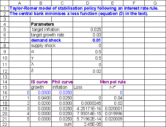
The adjustment path is described by the triangle in Figure 1. Initially, growth increases but inflation does not change due to the lag in (2). The lag is explained by staggered price-setting by firms who have market power. The deviation of growth from its potential level causes inflation to rise, from (2). The central bank responds by increasing the interest rate according to the solution to its loss function and shown in the column, r-r*, in the spreadsheet. This in turn lowers growth, from (1). The lower output slows down the increase in inflation until the economy has moved to the top left point in the triangle in Figure 1. Note that growth has overshot its potential from high to low. This allows inflation to fall, from (2) which allows the central bank to lower interest rates. This process of falling inflation, falling interest rates and rising growth continues until the economy has returns to its initial equilibrium. This describes a boom-bust cycle, which is typical of the actual path of economies following a positive demand shock.
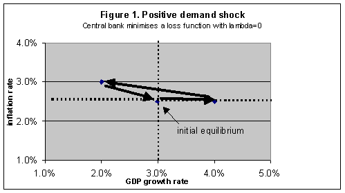
A simple extension is to allow the deviation of growth from potential to have a positive weight in the central bank's loss function. That is, l>0 in (3). The effect is to moderate the speed with which inflation returns to its target because now the growth rate is a consideration. This is illustrated in Figure 2 for the case of a 1% negative demand shock. The simulation is conducted by simply changing the entry for "demand shock" in the spreadsheet from plus to minus 1%.
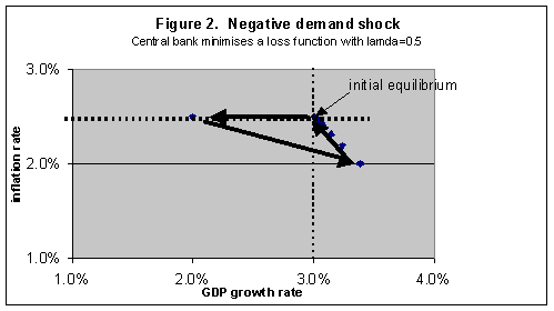
An important limitation of monetary policy is its inability to restore growth to its potential in the face of a sustained negative supply shock. A good example of a sustained negative supply shock is an oil price shock that gets embedded in a wage-price spiral. This can be clearly and simply demonstrated by replacing "demand shock" with "supply shock" in the spreadsheet. An example is shown in Figure 3.
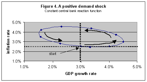
Another worthwhile extension is to relax the assumption that the central bank sets interest rates by minimising a loss function under perfect foresight. In practice, interest rate decisions are made in an environment of inherent uncertainty. Hence the central bank's reaction function is determined in a less mechanistic way, reflecting judgement, experience, a feel for the data, and so on, rather than as the solution to a loss minimising problem. To capture this process we can specify an ad hoc monetary policy reaction function of the form:
(4) rt = r* + s1(pt - p*) - s2(gt - gt*)
with exogenous values for the parameters s1 and s2 set initially equal to 2 and 0 respectively (s2=0 implies an inflation-only target which is the maintained assumption throughout the analysis in this paper). Such a reaction function is implied by the minimisation approach above but with time varying parameters s1 and s2. The resulting adjustment path for a positive demand shock of 1% is shown in Figure 4. The path follows an elliptical pattern. The parameter values were chosen so that the path returns to its initial equilibrium point. However, simulations showed that this is a special case. There is a range of paths, which do not return to the initial point; some are stable paths spiralling inward and some are unstable paths which spiral outward. Students can easily experiment with different parameter values. The general point that these simulations illustrate is that stabilisation policy (like all economic policy) is not an exact science. This can be more vividly illustrated by extensions to the above exercises, such as simultaneous supply and demand shocks.
Evidence has been steadily accumulating that economics students would achieve higher quality learning outcomes with more emphasis on applying economic theory to real world problems (Guest and Duhs 2002; Colander, 2000; Heyne, 1995; Siegfried et al., 1991). Achieving this goal requires a readiness on our part to replace models that no longer describe real-world economic mechanisms, or that do so in an overly-complicated way. This has been the case with the LM curve as a tool for teaching monetary policy since the adoption of an interest rate rule by almost all central banks of industrialised countries. This article has shown how the Taylor-Romer model, a more realistic and simpler alternative, can be taught in very hands-on way. The spreadsheet approach demonstrated here is suitable at the Principles level, which is the right time to introduce a real world, hands-on approach to learning economics.
This Appendix provides the derivation of the growth form of the IS curve (1) and the Phillips curve (2).
The Phillips curve can expressed in terms of inflation and unemployment as follows (symbols are as defined in the text unless indicated):
(A1) pt = pt-1 + f(ut - ut*) + wt
where u is the unemployment rate, u* is the NAIRU (note5). It is assumed that pt-1=p*, where p* is the expected rate of inflation and expectations are backward looking. We then invoke Okun's Law, which relates the change in the output growth gap to the unemployment gap as follows:
(A2) ut = ut* + q(gt-1 - gt-1*) + dt
where g is the growth rate of output and g* is the output growth counterpart of the NAIRU (note6). Substituting (A2) into (A1) we have the Phillips curve equation (2) in the text:
p = pt-1 + a(gt-1 - gt-1*) + et
(A3) yt = yt* + s(rt-1 - r*) + mt
where y and y* are the level of output and potential output, respectively, and r is the real interest rate. Define the growth rates for output and potential output as follows:
(A4) yt* = yt-1*(1 + gt*)
and
(A5) yt = yt-1(1 + gt)
where g and g* are the growth rate and potential growth rate, respectively. Substituting (A5) and (A4) into (A3), and assuming yt-1=yt-1* for t=1 (note7), gives:
(A6) 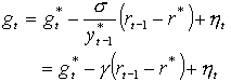
1. Solver is an Add-In, which may need to be installed (select Add-Ins from the Tools menu).
2. This model is given in Debelle (1999), the only difference being that Debelle adopts the conventional approach of expressing output in levels rather than growth rates. Taylor (2000) also expresses output in levels form; and he wrote down the interest rate policy function directly as the third equation instead of specifying the loss function from which the interest rate function is derived.
3. The "neutral" interest rate means the interest rate where inflation and output are equal to their targets.
4. The expectation sign in the loss function is ignored by assuming that the central bank has perfect foresight and that shocks are unanticipated.
5. The NAIRU is the non-accelerating inflation rate of unemployment.
6. This can be described as the maximum rate of output growth that can be achieved with a steady inflation rate.
7. For t>1 there will be lags in the rt process in (A6), but (A6) serves as a satisfactory approximation for pedagogic purposes.
Cahill, M. B. and Kosicki, G. (2001), "Using Spreadsheets to Explore Neoclassical Assumptions in a New Keynesian Model", CHEER, 14, 2
Debelle, G. (1999), "Inflation Targeting and Output Stabilisation", RDP 1999-08, Reserve Bank of Australia.
Guest, R. and Duhs, A. (2002) "Economics Teaching in Australian Universities: Rewards and Outcomes", The Economic Record, 78 (240)
Heyne, P. (1995), "Teaching Introductory Economics", Agenda, 2(2): 149-158.
King, R.G. (2000), "The New IS-LM Model: Language, Logic, and Limits", Federal Reserve Bank of Richmond Economic Quarterly, 86/3.
Reserve Bank of Australia (RBA) (2001), "Monetary Policy in Australia", http://www.rba.gov.au/PublicationsAndResearch/Education/Monetary_Policy_In_Australia.html#object
Romer, D. (2000), "Keynesian Macroeconomics Without the LM Curve", Journal of Economic Perspectives, 14, 2, 149-169
Siegfried et al (1991), "The Economics Major: Can and Should We Do Better Than a B?", American Economic Review, 81(2): 20-25.
Taylor, J. (1998), Principles of Macroeconomics, 2nd Edition, Houghton Mifflin Company, Boston.
Taylor, J. B. (2000), "Teaching Modern Macroeconomics at the Principles Level", AER Papers and Proceedings, 90, 2, 90-94
Ross Guest