Forecast Evaluation using Theil’s Inequality Coefficients

Alternative Specifications and Their Properties

Summary

Forecast evaluation is a central topic in the teaching of forecasting. Located within the battery of statistics available for forecast evaluation are Theil’s Inequality Coefficients. However, while the inclusion of these statistics within forecasting modules is undeniably important, it can be problematic as their presentation in textbooks and software packages fails to adequately reflect the alternative specifications available along with their differing properties and the associated literature. This case study addresses these issues concerning specifications, properties and existing research. This insight into the nature of Theil’s statistics is increased further via the provision of an interactive Excel file which presents examples to illustrate the differing issues raised. The Excel file has the additional benefit of allowing readers to automatically calculate the various statistics for examples of their choice.

Potential Confusion Concerning Theil’s Inequality Coefficients

The application and interpretation of forecast evaluation statistics occupies an undeniably vital position in the syllabi of forecasting modules. Amongst the range of alternative statistics available for consideration are Theil’s Inequality Coefficients. However, incorporation of Theil’s statistics within the delivery of forecasting modules is complicated as a result of a number of interrelated issues which can potentially hamper understanding of their properties. These issues include the following.

• There are two specifications for Theil’s Inequality Coefficient. The presence of these two forms, which can be denoted as U₁ and U₂ respectively, can itself generate some confusion. This is compounded by the fact that some texts consider just one of the specifications and hence potentially leave readers under the impression that only a single form exists. For example, while Pindyck and Rubinfeld (1997) presents U₁ only, the classic forecasting text of Makridakis et al. (1998) contains discussion of just U₂.
   
• Aside from obvious differences in their construction, the interpretation of the statistics differs. While U₁ is bounded between 0 and 1, U₂ has a lower bound of 0 but instead considers 1 as ‘threshold’ value which indicates a forecasting performance equivalent to that of the naïve forecasting approach. Values either side of 1 therefore provide evidence on forecasting accuracy relative to the naïve approach, with U₂ < 1 indicating a degree of forecasting accuracy greater than the naïve method and U₂ > 1 indicating that the forecasts under consideration are less accurate than those offered by the naïve method.
   
• A number of papers exist which consider the relative robustness or merits of the alternative U₁ and U₂ specifications. Prominent studies within this literature include Bliemel (1973), Granger and Newbold (1973) and Ahlburg (1984). In summary, these studies discuss a preference for the use of U₂ over U₁ due to limitations associated with the latter. However, presentation of U₁ often occurs without reference to these studies and the relevant information they provide. Again, this can result in confusion or uncertainty regarding their application and their associated degrees of robustness.
   
• Beyond the alternative forms of Theil’s inequality coefficient, there are further associated ‘Theil’ statistics available in the form of three proportions arising from the decomposition of the (squared) numerator of the U₁ specification. Not only does this decomposition lead to further statistics being available for consideration, but the associated literature presents two alternative specifications of these three sets of proportions. So, potential confusion can arise as there are further statistics to consider which can themselves be specified in different ways! The issue is complicated further as debate on these decomposition statistics has led to one specification being identified as preferable while the other presented in software.

In summary, while it is important to incorporate Theil’s inequality coefficient within the syllabus of forecasting modules, there are numerous complicating factors which arise as a result of the availability of alternative specifications with differing properties, the presence of alternative definitions for associated proportions which themselves have different properties, and differing and incomplete presentations of the statistics and associated literature within textbooks and software packages. To address the potential confusion this might generate for those wishing to provide a more complete presentation of the statistics in their teaching, the following section provides a discussion of the mechanics, interpretation, properties and relevant literature associated with the statistics. This is supplemented in the section thereafter by the presentation of an interactive Excel file to provide illustrative examples to reinforce the discussion and allow practitioners to create further solved examples.

Alternative Specifications and Statistics

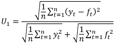
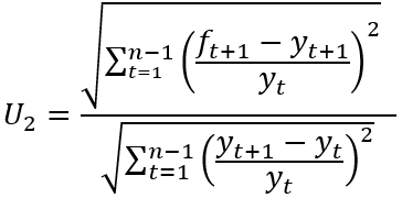
Given n observations on a variable of interest denoted as y_t and a set of associated forecasts denoted as f_t, the two specifications of Theil’s inequality coefficient U₁ and U₂ can be denoted as below:

(1) 

(2) 

As noted above, these statistics differ in terms of their construction and interpretation. Considering U₁, this is a (0,1) bounded statistic, with perfect forecasting (i.e. y_t = f_t ∀ t) resulting in U₁ = 0. Larger values of U₁ approaching the upper bound of 1 are then typically argued to indicate increasingly inaccurate forecasts. However, the limitations of this statistic have been discussed by Bliemel (1973) and Granger and Newbold (1973). For example, it can be seen that U₁ = 1 will be observed should one of y_t or f_t equal zero in all periods. To illustrate this limitation, consider a hypothetical situation in which a set of forecasts takes the value zero throughout the forecast period while y_t takes non-zero values. In these circumstances the numerator and denominator of the statistic become equal and U₁ = 1 will result irrespective of the values of y_t and the proximity of f_t to these values. Consequently, it is possible, for example, for one set of near zero forecasts to return a greater value for the U₁ statistic than an alternative less accurate set of forecasts which are further from the value being forecast in every period considered.

The U₂ statistic has a different interpretation. While perfect forecasting (i.e. y_t + 1 = f_t + 1 ∀ t) produces a value of zero for this statistic, the value of 1 represents a threshold where forecasting accuracy is equivalent to a naïve, or no change, forecast. From inspection of (2) it can be seen that a naïve forecast (which involves f_t + 1 = y_t) results in the numerator and denominator of this expression being equal and hence U₂ = 1. Values above (below) 1 are then taken to indicate a forecasting performance which is less (more) accurate than the naïve approach. In contrast to the criticism faced by the U₁ statistic, the U₂ statistic receives support in studies such as Bliemel (1973), Granger and Newbold (1973) and Ahlburg (1984). However, as noted above, the presence of two specifications and the discussion of their relative properties are not always noted when Theil’s statistic is presented in textbooks and software.

To assess different aspects of forecasting accuracy, ‘proportions’ of Theil’s U₁ statistic have been proposed. These proportions are based upon the (squared) value of the numerator of (1). However, to complicate matters (!), two decompositions of this expression have been suggested. The first set of proportions arises from the following decomposition of the (squared) numerator of (1):

(3) 

Using the terminology of, inter alia EViews 9.5, this leads to the bias (U^M), variance (U^S) and covariance (U^C) proportions:

(4) 

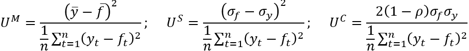
where { ȳ, f̄, σ_y, σ_f, ρ } denote the mean of the actual value, the mean of the forecasts, the standard deviation of the actual values, the standard deviation of the forecasts and the correlation between the forecasts and actual values, respectively. The interpretation placed upon these statistics is that the bias proportion U^M examines the relationship between the means of the actual values and the forecasts, U^S considers the ability of the forecast to match the variation in the actual series, and U^C captures the residual unsystematic element of the forecast errors. By construction, U^M + U^S + U^C = 1 with the stated preferred outcome for these statistics being values as close to zero as possible for U^M and U^S, with U^C consequently being as close to 1 as possible.

The alternative set of proportions which has been proposed is based upon the following decomposition:

(5) 

This decomposition leads to the following proportions:

(6) 

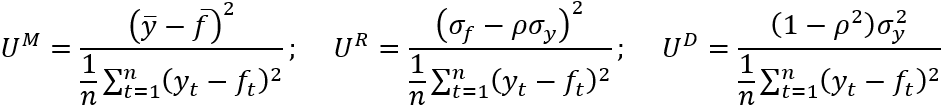
While it can be seen that this alternative decomposition leads to the production of the same bias proportion (U^M), new regression (U^R) and disturbance (U^D) proportions arise. Granger and Newbold (1973) consider the relative merits of the two sets of proportions. The arguments presented lead to a preference for the second set of proportions { U^M, U^R, U^D }. In particular, via general discussion and an illustrative specific example, Granger and Newbold (1973) question the merits of U^S, presenting arguments against the expectation of an equality between the standard deviations of a series and an optimal forecast of it.

Illustrative Examples

To allow calculation of the above two Theil Inequality Coefficients and the two alternative sets of proportions, the Excel file Theil.xlsx has been created. This spreadsheet contains a simple example involving 10 observations on two alternative sets of forecasts (denoted as f1 and f2) of a variable of interest (denoted as y). The spreadsheet is populated with hypothetical values for these series to illustrate various properties of the alternative statistics considered. However, these values can obviously be replaced to calculate results for other series.

The currently included values present a variable of interest (y) which alternates between the values –1 and 1. As noted, hypothetical values are included in this example for illustrative purposes. However, this could be considered as an extreme version of a series which fluctuates around zero such as a measure of changes in inventories. The two sets of forecasts f1 and f2 also take hypothetical values, with f1 taking the value of 0 in all but the final period and f2 alternating between under- and overprediction. The above Theil statistics and proportions are presented for f1 and f2, along with the mean square error (MSE) which provides an alternative measure of forecast accuracy. The results in the Excel file are reported below in Table One.

Table One: Forecast Evaluation Statistics

Statistic	f1	f2
U1	0.9601	0.5000
U2	0.4967	1.0000
MSE	0.9810	4.0000
UM	0.0001	0.0000
US	0.9591	1.0000
UC	0.0408	0.0000
UR	0.0938	1.0000
UD	0.9061	0.0000

The results in Table One illustrate a number of the issues raised above concerning the properties of the statistics considered. Issues to consider include:

• From inspection of the spreadsheet, the errors associated with f1 are clearly smaller in absolute terms that those associated with f2 in every period. This is reflected in the resulting values of the MSE and U₂ which lead to f1 being preferred to f2. However, the values for U₁ suggest the opposite, with U₁ = 0.9601 for f1 compared to U₁ = 0.5 for f2. These findings demonstrate the above discussion of the impact of zero values for either the series of interest or its forecasts upon U₁. In this case, f1 takes a value of zero in all but one period and hence returns a larger value of U₁ than the alternative set of forecasts f2 which has larger absolute errors. This demonstrates the noted limitation of the U₁ statistic.
   
• The alternative specifications of the proportions of Theil’s statistic can be seen to generate markedly different values for f1. While the bias proportion (U^M) is common to both sets of proportions, the value of variance proportion in the first specification (U^M = 0.9591) differs markedly from the value of the regression proportion (U^R = 0.0938) in the second specification. Similarly, the values of the covariance (U^C = 0.0408) and disturbance (U^D = 0.9061) proportions differ. The differing values of U^S and U^R reflect the inclusion of the correlation between the series of interest and its forecasts (denoted as ρ) in the latter but not the former. The spreadsheet calculates the correlation between a series and its forecasts, returning a value of ρ = 0.3333 for y and f1. This correlation has a dramatic impact in the present example where the standard deviation of y is much greater than the standard deviation of f1. While these are compared directly in U^S, the impact of the higher variance of y is mitigated in U^R via its multiplication by ρ. Consequently, the large value of U^S = 0.9591 contrasts markedly with U^R = 0.0938.
   
• The results for f2 show that its perfect positive correlation (ρ = 1) with y (note f2 = 3y), leads to U^S = U^R. Similarly, ρ = 1 leads to U^C = U^D = 0 as this results in (1 – ρ) = 0 and (1 – ρ²) = 0 respectively.
   
• With the spreadsheet in place, further examples can be considered. For example, a further set of forecasts (f3) can be considered, which is given as f3 = –f2. This will generate a perfect negative correlation with the actual series (y) and the impact of this on the resulting statistics can be examined. For example, the ensuing difference between U^S and U^R can be discussed.

Conclusion

This case study has addressed potential confusion concerning the use of Theil’s Inequality Coefficient which might arise due to the existence of alternative specifications, differing properties, neglected insights from the literature and contrasting presentations of material in textbooks and software packages. It is hoped that the presentation offered herein and its support via an interactive spreadsheet will assist a more complete inclusion of these statistics within forecasting modules.

References

Ahlburg, D. (1984). Forecast evaluation and improvement using Theil’s decomposition. Journal of Forecasting, 3, 345-351. https://doi.org/10.1002/for.3980030313

Bliemel, F. (1973). Theil’s forecasting accuracy coefficient: A clarification. Journal of Marketing Research, 10, 444-446. https://doi.org/10.2307/3149394

Granger, C. and Newbold, P. (1973). Some comments on the evaluation of economic forecasts. Applied Economics, 5, 35-47. https://doi.org/10.1080/00036847300000003

Makridakis, S., Wheelwright, S. and Hyndman, R. (1998). Forecasting: Methods and Applications (3^rd edition). New York: Wiley.

Pindyck, R. and Rubinfeld, D. (1997). Econometric Models and Economic Forecasts (4^th edition). London: McGraw-Hill.

↑ Top