Flipping the Lid on Economics: Making Diminishing Returns Visible

Introduction

The aim of this case study is to demonstrate how I deliver a topic that is completely unfamiliar to first-year students from non-economics backgrounds in microeconomics seminars. It focuses on introducing the concept of diminishing marginal returns, which most students have never previously studied or even heard of before, through a role-play simulation. In this session, I also explain the related concepts of total physical productivity (TPP), average physical productivity (APP), marginal physical productivity (MPP), average cost (AC), and marginal cost (MC). Finally, I focus on the relationships between APP and AC, and between MPP and MC over time, using a tangible method that incorporates a transparent lid as a visual and practical tool to make these abstract concepts easier to understand.

Why I Selected These Methods

The main reason for choosing these particular teaching methods, such as the administrative staff role play and the lid analogy, is to bridge the gap between theoretical concepts and real-life understanding. Many of our students come in with limited background knowledge, and just looking at numbers or tables alone does not make the concept of diminishing marginal returns come alive for them. By going beyond standard teaching materials and using these relatable, everyday analogies, I aim to help students see how the theory applies to real situations. This makes it easier for them to engage, participate, and truly grasp the main learning objectives.

The University Administrative Office Simulation: Demonstrating Diminishing Marginal Returns

In this activity, I use a role-play simulation to actively engage with a group of students in the classroom. Each student is assigned the role of a university administrative staff member, and I act as their supervisor allocating tasks and resources. This approach transforms a traditional explanation into an interactive mini-drama, where students participate directly in the learning process. By assigning roles and narrating the scenario, I help them visualise the relationship between labour and output as we add more workers to a fixed number of laptops. The role-play structure keeps students attentive, encourages participation, and allows them to experience the concept of diminishing marginal returns.

I begin by telling the class: “Imagine we are running an admin office at a university, and we only have three laptops available in the office.” I then turn the explanation into a role play simulation. I select a group of five students from the class and engage each one individually by making eye contact. I tell them that I will employ them one by one as administrative staff members. The first three students, acting as administrative staff, each receive a laptop, while the last two staff members do not have laptops directly assigned to them. Instead, they are permitted to use the laptops only when their colleagues take a break. I also explain that their task is to carry out some administrative work for undergraduate and postgraduate level programmes by typing documents on the laptops, with their output measured by the number of pages they complete. This interactive and relatable approach sparks students’ curiosity and keeps them actively engaged throughout the exercise.

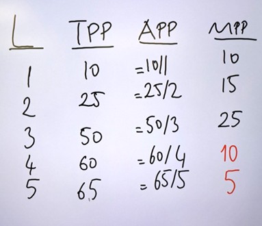
At this stage, I intentionally avoid using terms such as physical capital and limited availability of physical capital to simplify the scenario for students, as the activity itself already includes an element of physical capital, represented by the laptops. After this explanation, I move to the first student and tell them that they are the first staff member, who by the end of the task has typed ten pages. To demonstrate this, I draw a table on the whiteboard with columns labelled, from left to right, number of employees as L, TPP, APP, and MPP. After entering Labour (L) = 1 and Total Physical Product (TPP) = 10 in the table, I introduce the concept of Average Physical Product (APP). I explain to the class that it is calculated like any other average value, by dividing the total output by the number of workers, that is, APP = TPP / L.

I then move to the final column, labelled Marginal Physical Product (MPP), and engage the first student directly by asking,
“What has changed in total production after I employed you?”

The student usually responds, “Ten pages.” I confirm their answer by saying, “Yes, that is correct, your individual contribution is ten pages, and this represents the marginal physical product. It shows how much total production increases when we add one more worker.”

This dialogue-based approach helps students actively connect the formula with its real meaning.

I continue the simulation with the second student and enter TPP = 25 in the table. I ask, “What has changed after employing you?” The student replies that they contributed an additional fifteen pages, which represents their marginal physical product (MPP). I then explain that this increase occurs because the second staff member focuses only on undergraduate level tasks, allowing for greater specialisation and teamwork.

I then continue the simulation with the third student and enter TPP = 50 in the table. I explain that this increase occurs because the third staff member focuses only on first year undergraduate programmes. By the end of the exercise, MPP rises to 25 pages, showing a larger contribution from the third worker compared with the previous ones as a result of greater specialisation.

Later, I move to the fourth student and explain that total productivity (TPP) has now increased to 60 pages, meaning their marginal contribution (MPP) is 10 pages. Finally, when I employ the fifth staff member, the TPP rises to 65 pages. Although this worker still contributes to output, their additional productivity is smaller than that of the previous worker, with an MPP of only 5 pages. I highlight to the class that the decline in the contribution of the last two staff members to total output is understandable, as they can only use the laptops when their colleagues are on break.

Figure 1. Calculating APP and MPP

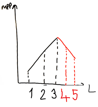
After finalising the table and completing all columns, including Marginal Physical Product (MPP), I draw the MPP curve on the whiteboard to illustrate the relationship between additional labour and their productivity. The horizontal axis represents the number of workers employed, while the vertical axis shows the marginal product. Using a black marker, I illustrate the first phase, where the MPP increases for the first three staff members and reaches its peak, reflecting the benefits of specialisation and teamwork. Then, using a red marker to indicate the turning point, I draw the second phase, where the MPP begins to decline after the fourth and fifth staff members are employed. I explain that this second phase marks the point at which diminishing marginal returns occur due to the limited availability of laptops.

Figure 2. The relationship between labour (L) and marginal physical product (MPP)

After illustrating diminishing marginal returns, I draw the Total Physical Product (TPP) curve to show the relationship between TPP, Marginal Physical Product (MPP), and Average Physical Product (APP), and to demonstrate how both MPP and APP can be derived from the TPP curve. For this purpose, I draw two red dashed lines from the origin to the TPP curve. The first line, which is the lower one, intersects the TPP curve at two points. The first intersection represents the point where MPP reaches its peak, corresponding to the steepest slope of the TPP curve, while the second intersection represents the point where MPP becomes zero and TPP reaches its maximum. The second line, which is the upper one, is tangent to the TPP curve and represents the point where APP reaches its maximum. At this tangency point, APP and MPP are equal. Finally, I explain that as MPP continues to decline, it eventually crosses APP from above at the point where APP reaches its peak and later becomes zero when the TPP curve reaches its maximum.

Figure 3. The relationship between Total Physical Product (TPP), Average Physical Product (APP), and Marginal Physical Product (MPP)

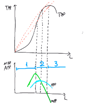
In both phases, Total Physical Product (TPP) continues to increase, but after the first phase, the additional output produced by each extra unit of labour begins to decline. This occurs because productivity is constrained by the fixed amount of physical capital, represented by the limited number of laptops available, which leads to diminishing returns. Moreover, at the end of the second phase, where Marginal Physical Product (MPP) becomes zero, the TPP curve reaches its peak. The subsequent stage represents the third phase of production, where TPP starts to decline and MPP becomes negative.

After teaching the fundamental concepts of productivity, I move on to explain the relationship between productivity and cost, specifically between Average Physical Product (APP) and Average Cost (AC), and between Marginal Physical Product (MPP) and Marginal Cost (MC), even though the topic of cost is scheduled to be covered in the following seminar. I believe that students should not view these two topics as separate; it is more effective to illustrate the relationship between them at this time, as otherwise they might overlook this important connection.

Use of a Semi-Transparent Lid

To help students grasp this link more easily, I begin from a broad perspective and ask a simple question about the relationship between productivity and cost. Students can quickly recognise that productivity and cost move in opposite directions.

I then link this understanding to Average Physical Product (APP) and Average Cost (AC), explaining that these two curves move in opposite directions, effectively behaving as mirror reflections of one another. Any change in Average Physical Product (APP) is reflected in the opposite direction by Average Cost (AC). The same principle applies to Marginal Physical Product (MPP) and Marginal Cost (MC).

To help students clearly visualise this connection, I use a semi-transparent lid that I borrowed from my kitchen. I ask students to follow along using a piece of paper and draw a U shaped smiling curve representing Average Cost (AC). Then, I ask them to draw another curve starting below the first one and intersecting the minimum point of the U-shaped curve. This second curve represents Marginal Cost (MC).

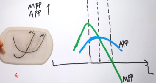
After everyone completes their drawing, I show my version drawn on the semi-transparent lid. At first, the students appear curious but unsure about its purpose. Then, I flip the lid upside down and hold it next to the APP and MPP diagram on the whiteboard (See Figure 4). They immediately notice that my smiling face illustration, along with the MC curve, matches the diagram on the board once it is flipped. At that moment, the connection becomes clear, and students realise that the two drawings share the same shape, visually reinforcing the inverse relationship between productivity and cost.

Figure 4. The use of a transparent lid to illustrate the inverse relationship between productivity curves (APP and MPP) and cost curves (AC and MC)

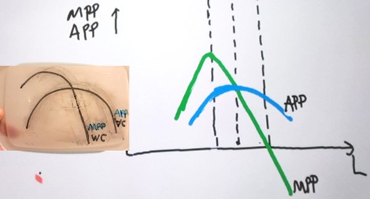
Then I flip it upside down again and let the students see a simple smiling face representing the AC curve and the MC curve, which I hold next to the APP and MPP curves on the board (See Figure 5). The students realise that the relationship between productivity and cost is indeed inverse. As APP rises, AC falls, and when APP begins to decline, AC starts to rise. When APP reaches its maximum point, AC reaches its minimum point. I then move to the relationship between MPP and MC and explain it in the same way. After establishing these relationships, I also highlight the correspondence between the productivity curves (APP and MPP) and the cost curves (AC and MC). I note that MPP intersects APP at APP’s peak, just as MC intersects AC at AC’s lowest point. Throughout this explanation, I maintain eye contact with the students to check their understanding, and I notice that the smiling faces are no longer only on the board but also on the faces of the students, showing both their engagement and the positive impact of this teaching method on their learning and satisfaction.

Figure 5. Visualising the mirror relationship between productivity and cost through the use of a transparent lid

Student Reflection

Students in my class expressed their satisfaction not only through their facial expressions and verbal feedback but also in their written comments. Several students highlighted the effectiveness of both teaching approaches, as shown below:

“The admin staff roleplay was a very good way to explain it; it made it easier to understand. Lid from kitchen was another good way to show it, so no improvements I can think of.”

“The role play was fun. Good to see it in a visual representation. I really like the lid analogy, very creative and smart. I liked the lid analogy the best.”

“I liked the admin staff scenario and it helped me to best understand the topic. The lid from kitchen still a useful way of learning but I preferred the other method.”

“I enjoy the interactive activities they help me engage with the content after a long day!”

“The administrative staff example was easy to understand and was a fun. The Lid From Kitchen was very good and helped to correlate between marginal production and marginal costs.”

Conclusion

Even though we teach the same topic, the way we deliver our classes and the innovative and creative methods we incorporate into our teaching significantly shape the quality of instruction and enhance students’ participation and engagement. Therefore, being proactive in selecting or creating the most appropriate teaching methods and materials is extremely important to ensure the quality of our work. As a result, students are more likely to achieve the intended learning objectives effectively.

More specifically, delivering abstract and unfamiliar topics requires particular attention when teaching first-year students, as this stage is crucial for their successful integration, academic development, and continued engagement in their studies. Considering these risks and weaknesses, teachers ought to either develop new ways of delivery or adopt existing methods, such as role play, the use of analogies, and the use of objects, and embed these into their teaching to promote student participation, engagement, and ultimately academic success.