Analysing Forecasting Bias: Significance, methods and samples

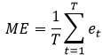
Forecasting bias is an obvious issue to consider when examining the properties of forecasts and forecasting methods. As a result, ‘bias’ is a standard feature on the syllabi of forecasting modules and in the contents of forecasting texts. When considering material on forecasting bias, there are two obvious ways in which this can be presented. First, the mean error (ME) for a set of forecasts can be considered.  Second, a more formal approach can be adopted via recourse to testing for bias, with the Holden-Peel (1990) test an obvious test to consider. The purpose of this study is, initially, to provide an empirical example of these approaches in practice. This will then allow consideration of where and how they coincide in terms of the information they provide and, importantly, how they differ. However, the analysis will also permit discussion of how the examination of bias can be sample specific and hence be dependent upon the interaction between the forecasting method employed and the nature of the data examined. Via empirical analysis, the relevance and importance of these issues will be illustrated to complement the standard presentation of forecasting bias considered in texts.

The Mean Error (ME) and Testing for Bias

Given a series of interest denoted as y_t and a set of forecasts of it denoted as f_t, where t = 1, ..., T, associated forecast errors can be generated as e_t = y_t - f_t. The ME can then be derived as below:

(1) 

While the ME is simplistic in nature, it has an advantage over more sophisticated forecast evaluation statistics such the mean square error or Theil’s inequality coefficient as it provides information on potential bias. With regard to interpretation, a negative ME obviously indicates overprediction on average, while a positive value indicates underprediction on average. However, it has to be recognised that while an average tendency towards bias can be inferred from the value of the ME, the statistic does not provide information on whether this bias is significant statistically. To assess whether bias is significant, the Holden-Peel (1990) test can be employed via consideration of the following regression:

(2) y_t - f_t = λ + u_t

where the null of no bias H₀: λ = 0 can be tested via a t-test. In common with the interpretation of sign for the ME statistic, a positive value for λ̂ indicates potential underprediction, while negative values indicate potential overprediction. Indeed, this identical approach to interpretation arises as λ̂ is equal to the ME by construction. However, while the ME statistic and bias coefficient return the same calculated value, the latter differs as it allows subsequent testing of whether the observed average under- or overprediction is significant. That is, a negative (positive) λ̂ or ME may be observed thus indicating potential overprediction (underprediction) but this value may not prove to be significant and hence significant bias will not be present. The following material will illustrative these issues via consideration of an empirical example.

An empirical analysis of forecasting bias

To consider the above issues concerning potential and significant bias, an empirical analysis of property crime in the USA is considered. The data are annual observations from 1960 to 2012 on the number of property crimes per 100,000 inhabitants in the USA and are available from the property.xlxs file.[1]  To produce forecasts, two methods are considered to generate a series of one-step ahead forecasts. The first is the naïve forecasting method where the forecast for the next period is simply the actual value observed in the current period. The second method is a third order moving average forecast, or MA(3), where the forecast for a given period is the average of the values in the three periods preceding it.

The results obtained from application of the Holden-Peel test using forecasts from the two methods are provided below.  To illustrate the impact of the application of the Holden-Peel test to differing sample periods, the tests are applied to the full sample of 1960-2012 along with three sub-samples relating to changes in the evolution of criminal activity noted in the literature.[2] In terms of sign and significance of forecasting bias, the two methods produce qualitatively similar results.  From inspection of the results for the naïve forecasting method, the values of λ̂ (and hence ME) can be either positive or negative depending upon the sample employed.[3] Hence potential underprediction or overprediction varies across the samples examined. Interestingly, analysis of the significance of potential bias produces varying results also.  From inspection of the reported p-values, significant bias is apparent in the first and third subsamples (namely the samples 1960-1980 and 1991-2012) where significant underprediction and overprediction, respectively, are observed. As noted, the findings for moving average forecasting are qualitatively similar to those for the naïve method.[4] These results therefore indicate that while the ME may indicate bias in the form of an average tendency, this may not be significant. Also, the findings illustrate that conclusions concerning bias may be sample-specific.

SAMPLE PERIOD	Naïve Forecasting		MA(3) Forecasting
	λ̂	p-value	λ̂	p-value
1960-2012	21.79	[0.45]	43.60	[0.38]
1960-1980	181.35	[0.00]	369.28	[0.00]
1981-1990	-28.02	[0.65]	-8.27	[0.94]
1991-2012	-100.63	[0.00]	-199.29	[0.00]

References

Box, G. and Jenkins, G. (1970) Time Series Analysis: Forecasting and Control. San Francisco: Holden-Day. ISBN: 0816211043

Holden, K. and Peel, D. (1990) ‘On testing for unbiasedness and efficiency of forecasts’, Manchester School, 58, 120–127. doi: 10.1111/j.1467-9957.1990.tb00413.x

---

[1] The data are available from http://www.ucrdatatool.gov/Search/Crime/State/StatebyState.cfm.

[2] In short, the criminology literature makes reference to a steady increase in crime until around 1980 where a plateauing was observed.  This was subsequently followed by a third epoch in which the 1990s witnessed a decline in crime.

[3] Note the two forecasting techniques considered are best suited to series which do not exhibit either trending or seasonal behaviour.  As a result, they, in a sense, serve as strawmen given their application to two sub-samples in which a general increase and a general decrease, respectively, are observed.  However, the motivation here is to demonstrate variation in findings concerning bias rather than identify the optimal forecasting technique for the series under investigation.

[4] Note that the two forecasting methods are not directly comparable for the full sample or first subsample due to the inclusion of different numbers of forecast errors.

↑ Top