Forecast Combination: A tool for teaching and demonstrating the underlying issues

When teaching forecasting at undergraduate or postgraduate levels to economics, business or finance students, a standard syllabus will contain topics such as the smoothing methods of Holt and Holt-Winters, and the ARIMA models of Box and Jenkins. As a result students are provided with a clear illustration, appreciation and mastery of alternative tools and techniques to produce forecasts for time series data. To allow recognition of the potential benefits to be gained from the combination of forecasts produced using different methods (as initially proposed by Bates and Granger, 1969), the variance-covariance of forecast combination is another standard component of such modules.

The underlying logic of the variance-covariance method of forecast combination is quite straightforward. In essence, and in its simplest form, it considers the possibility that when considering two rival forecasts each may provide information not present in the other. As a result, a combined forecast drawing upon them can prove a ‘better’ forecast than each of the individual component forecasts. However, while the motivation underlying forecast combination is quite intuitive, the associated algebra can prove less accessible. As a result, I have developed an Excel spreadsheet to illustrate and demonstrate the relevant issues associated with the approach in a (perhaps) more transparent and visual manner.

Coverage of forecast combination is provided in a number sources, including Holden et al. (1985) and Clements and Harvey (2010). Given the definite structure of this topic, the following draws upon the presentation provided in the above sources. Consider a variable of interest denoted as y_t, and two sets of unbiased forecasts of it denoted as f_1t and f_2t respectively. Formally, these forecasts can be presented as:

1) y_t = f_1t + e_1t

2) y_t = f_2t + e_2t

where E[e_it]=0 and V[e_it]= σ_i²; for i = 1,2. The combined forecast, denoted as f_t^c, is then given as:

3) f_t^c = (1 - λ)f_1t + λ​f_2t

Obviously the combined forecast is unbiased given it is the weighted sum of two unbiased forecasts with weights that sum to unity. The appropriate value of λ, and hence the values of the weights, is determined via minimisation of the mean square forecast error (MSFE) associated with the combined forecast.  To achieve this, the MSFE of f_t^c is differentiated with respect to λ. With MSFE specified as:

4) MSFE[f_t^c] = (1 - λ)σ₁² + λσ₂² + 2λ(1 - λ)σ₁₂

As the covariance between the errors of the individual forecasts is equal to the product of their correlation and their standard deviations (that is, σ₁₂ = ρσ₁σ₂), the above expression can be re-expressed as:

5) MSFE[f_t^c] = (1 - λ)σ₁² + λσ₂² + 2λ(1 - λ)ρσ₁σ₂

The resulting ‘optimised’ value of λ (denoted as λ*) is then given as:

6) 

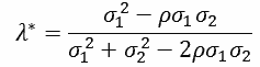
As shown by, inter alia, Clements and Harvey (2010), the above value of λ* can be substituted into the above expression for MSFE[f_t^c] to derive the minimum MSFE for f_t^c. Formally, this can be expressed as:

7) 

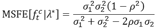
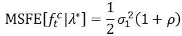
Further to this, and as depicted clearly by Clements and Harvey (2010), if ρ ≠ 1 gains from forecast combination are possible even when the underlying forecasts have errors with equal variances. This is apparent from substitution of σ₁²​ = σ₂² into (7) which results in:

8) 

As can be observed from the above discussion, understanding of the nature of forecast combination can be masked quite easily by a wealth of associated algebra. However, the underlying issues that need to be recognised, and which support and allow understanding of the above formal representation, are quite intuitive. To aid and encourage such learning, I have created an Excel spreadsheet to permit both experimentation with the above components and graphical depiction of resulting outcomes for MSFE[f_t^c]. Using the spreadsheet, alternative values of {σ₁², σ₂², ρ} can be considered with the resulting values of MSFE[f_t^c|λ*] and λ* calculated automatically. In addition, all values of MSFE[f_t^c] are calculated for all values of λ in the range (0,1). Therefore, use of the spreadsheet and consideration of alternative values of {σ₁², σ₂², ρ} allows a range of important issues concerning forecast combination to be considered, including:

• Demonstration of the possibility of gains from forecast combination, in terms of  being lower than the error variances for the individual forecasts, when ρ < 1.
• Demonstration of the inverse relationship between the optimised weights, (1 - λ*) and λ*, attached to individual forecasts and the variances of their associated errors.
• Demonstration of the increased gains from combination as ρ →-1.

To illustrate the above, consider the results obtained when the initial values provided in the spreadsheet, {σ₁2, σ₂², ρ} = {2, 12, -0.6} are employed. As can be seen, this results in MSFE[f_t^c|λ*] = 0.77 and λ* = 0.25. From this, it can be seen that:

• The negative value of ρ results in a lower MSFE for the combined forecast than the error variances of the individual forecasts (0.77 compared to 2 and 12).
• The weighting attached to the first forecast is far greater than that attached to the second forecast (0.75 compared to 0.25). This demonstrates the inverse relationship between the weights and the error variances.
• MSFE[f_t^c] falls towards its minimum value as the weighting on the second forecast approaches its optimised value of 0.25. This reduction depicts an offsetting effect between the forecasts which is analogous to the diversification effect in portfolio theory.

References

Bates, J. and Granger, C. (1969) ‘The combination of forecasts’, Operations Research Quarterly, 20, 451-468.
https://doi.org/10.2307/3008764

Clements, M. and Harvey, D. (2011) ‘Forecast combination and encompassing’, in Mills, T. and Patterson, K. (eds) The Palgrave Handbook of Econometrics, Volume 2: Applied Econometrics, Oxford: Palgrave. ISBN 9781403917997

Holden, K., Thompson, J. And Peel, D. (1985) Economic Forecasting, Cambridge: Cambridge University Press. ISBN 9780521356923