Directional Forecasting, Forecasting Accuracy and Making Profits

Synopsis

This case study aims to provide a discussion of directional forecasting and its importance in the teaching of forecasting at undergraduate and postgraduate levels. It could be argued that directional forecasting receives insufficient attention at present given its infrequent inclusion in the delivery of such modules, its limited coverage in textbooks and the absence of tests for its presence in many popular econometric software packages. As a consequence, the objectives of this case study are twofold. First, this study seeks to explain the nature of directional forecasting and its importance alongside conventional forecast evaluation procedures in the teaching of forecasting. Second, the study provides a worked example and a prepared Excel file to allow application of (arguably) the central test on directional forecasting proposed by Pesaran and Timmerman (1992).

Note: the Excel file has been updated in May 2018 to fix a typographical error.

Directional Forecasting

Forecast evaluation statistics are a familiar component of courses on forecasting in economics, finance and business.  Consideration of, inter alia, the mean error and mean square error through to more complicated statistics such as Theil’s U coefficients allows the relative strengths of alternative sets of forecasts to be examined.  The underlying message from this ‘typical’ analysis is a clear and has an intuitive appeal:  accuracy is good, inaccuracy is bad.  However, what does ‘accuracy’ mean when considering such statistics?  Clearly, it refers to point accuracy, and relates to forecasts being close to the values of the underlying series of interest.  While this property has an inherent usefulness in a variety of situations, it is often important when considering economic and financial series to be able to predict market movements, and the ability to predict movements does not necessarily coincide with ‘accuracy’ as defined above.  To illustrate this, consider an extreme, hypothesised example in which the change of a series is being forecast.  Suppose that upon examination a variable has been found historically to have increased by 0.5 units in every period.  Further to this, suppose that two sets of forecasts were generated for this variable (denoted as A and B) and these predicted a decrease of 0.5 units in every period (forecast A), and an increase of 100.5 units in every period (forecast B).  Which is then the more accurate set of forecasts?  Obviously the errors associated with the forecasts are vastly different with A having an (absolute) error of 1 unit and B having an error of 100 units.  In very crude terms, typical forecast evaluation statistics will lead to A being viewed as ‘better’ than B (obviously the respective mean errors are 1 and -100, while the respective mean squared errors are 1 and 10000).  However, suppose the crucial issue is predicting the movement in the market so that an investor can decide upon whether to sell (go short on) or buy (go long on) a futures contract.  In this case where market movement matters, B is the preferred forecast as it predicts correctly the direction of change.  Although this is a very simplified and extreme example, it does illustrate that accuracy in terms of predicting direction and returning ‘small’ errors will not necessarily coincide.

Given the importance of directional forecasting as a result of the frequent desire to know of market movements, it is perhaps surprising that this topic receives limited attention in the delivery of modules on forecasting.  This limited attention is more surprising given the work of Leitch and Tanner (1991) which provides an explicit discussion and empirical analysis of the profitability of economic forecasts.  In summary, the results of Leitch and Tanner (1991) show that profit has a stronger and more significant relationship with directional accuracy than accuracy as measured by conventional forecast evaluation statistics.  When considering the reasons for the lack of prominence of directional forecasting in forecasting modules, the availability of appropriate test to implement and illustrate the required analysis may be a potential factor.  For example, arguably the most prominent test for directional forecasting is that of Pesaran and Timmermann (1992).  However, despite its familiarity in the literature, the test is not incorporated in all econometric software packages.^{[note 1]}  Conscious that the limited availability of an appropriate test in an accessible manner may restrict coverage of the directional forecasting when teaching, this case study proceeds to provide a worked Excel file which allows calculation of the Pesaran-Timmermann test for a variable and an associated forecast.  In addition, the spreadsheet provides two applications to further illustrate the notion of directional forecasting and its relationship to conventional forecast evaluation statistics.

The Pesaran-Timmermann Test

Pesaran and Timmermann (1992) present a non-parametric test to examine the ability of a forecast to predict the direction of change in a series of interest.  Denoting the series of interest as y_t and the forecast of it as x_t, the proposed test is defined as:

(1) 

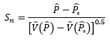
where:

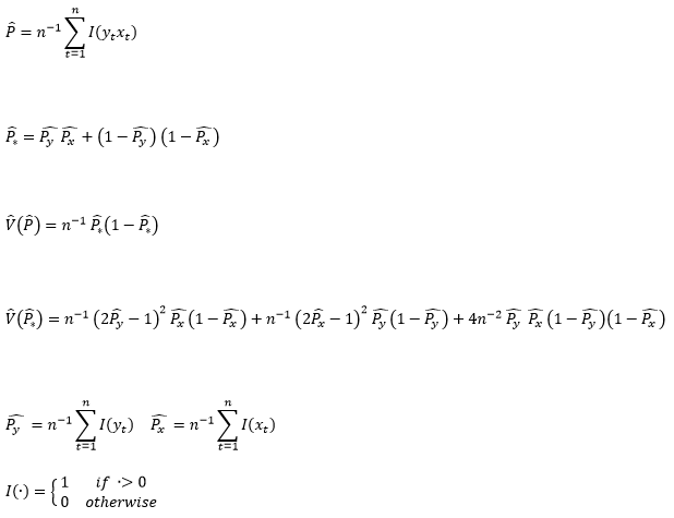
Under the null hypothesis of x_t not being able to predict y_t, S_n follows the standard normal distribution.

To permit application of the test and illustrate its use, the Excel file available via this link has been provided.  The file contains two spreadsheets each containing 100 observations of an artificially generated series of interest (Y) and a forecast of it (F1 in the first sheet, F2 in the second).  The spreadsheets return values for the S_n test statistic along with calculated mean error (ME) and mean squared error (MSE) statistics associated with the forecasts.  The results in the two spreadsheets are summarised in Table One below:

Table One: Forecast Evaluation Results

Forecast	ME	MSE	Sn
F1	-0.19	11.22	0.75
F2	42.41	44557.97	10.05

The results presented in the above table are straightforward to interpret.  While F1 can be seen to be more accurate than F2 according to the mean error and mean square error statistics (i.e. it returns lower values for both), the null associated with S_n is rejected when considering F2 but not when considering F1.  This illustrates the arguments of Leitch and Tanner (1991) in that while F2 may be less accurate in terms of standard forecast evaluation measures, it is to be preferred to F1 when the sign of a series (or the movement) is of importance.  Using the spreadsheets provided and making any (straightforward) adjustments required for the dimensions of the series, the S_n can be calculated for further variables.

References

Leitch, G. and Tanner, E.  (1991) ‘Forecast evaluation: Profits versus the conventional error measures’, American Economic Review, 81, 580-590. JSTOR 2006520

Pesaran, M. and Timmermann, A.  (1992) ‘A simple nonparametric test of predictive performance’, Journal of Business and Economic Statistics, 10, 461-465. https://doi.org/10.1080/07350015.1992.10509922

↑ Top