The Use of Cobb-Douglas and Constant Elasticity of Substitution Utility Functions to Illustrate Consumer Theory
This case study highlights the use of Microsoft Excel to present the derivation of compensated and uncompensated demand curves. It shows how a change in a good's price affects the quantity demanded of the good (and that of the other, composite good). It also shows how a change in income affects the quantity demanded of both goods. Excel's Solver Tool makes the development of consumer theory quite straightforward. The analysis is presented using a Cobb-Douglas utility function and a constant elasticity of substitution (CES) utility function. (The Cobb-Douglas utility function is more generally used and is a special case of the CES utility function.)
We make three contributions. First, we provide an explicit connection between the form of the utility function and the graphical presentation of the indifference curves, budget constraints (compensated and uncompensated), and demand curves (compensated and uncompensated). The CES utility function is given by:
U = A[aX-r + (1 - a)Y-r]-1/r . (1)
The Excel workbook lets the user select A and a. Rather than define r directly, however, the user specifies the elasticity of substitution, s. The exponent r is defined as (1-s)/s with a default s of 1.01. As s approaches 1, the function approaches the Cobb Douglas function; as s approaches 0, the function approaches the Leontief fixed-coefficient function; and as s becomes very large, the production function exhibits linear isoquants (X and Y are perfect substitutes).
Second, we make available to students, who are less comfortable with abstract models, a hands-on method of connecting utility functions to demand curves and decisions to buy a good. This is accomplished through a sequence of excel worksheets that develop a utility function, derive corresponding indifference curves, and maximizes utility though the use of Excel's Solver Tool. The use of scroll bars throughout the workbook allows students to observe and understand the effect of changing any of the parameters on the consumer's choice of quantity for both goods.
Third, we compare the results of the generally used Cobb-Douglas utility function (a special case of the constant elasticity of substitution function, the formula for which is Q = ALaKb), to those of the constant elasticity of substitution function. The CES function shares the Cobb-Douglas function's homogeneity of degree one. This causes the income-consumption curves to be rays through the origin. Also, the income elasticity of demand is unity for both products. The Cobb-Douglas function is restrictive in an additional way: its price consumption curve is horizontal, with the resulting unit price elasticity of (uncompensated) demand. The amount of Good is independent of the price of Good X, as are income shares for X and Y. The CES formulation does not share this restriction. As indicated in the figure below, the quantities of both goods now depend on relative prices as well as money income. In the case used for illustration, s exceeds unity and the price-consumption curve slopes downward.
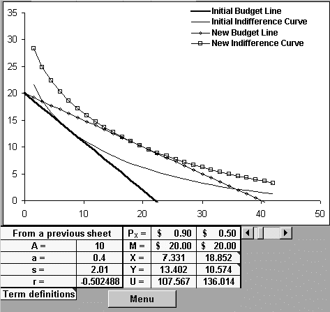
Figure 1: The Effect of a Price Reduction
The workbook proceeds to break the effect shown above into the effect due to substitution and that due to the impact of the price change on real income. It phrases the information above and that related to the above-described decomposition in terms of the compensated and uncompensated demand curves.
Either of the authors will provide the full workbook along with expanded discussion in response to an email enquiry.