Forecast encompassing tests as a means of forecast comparison

1. Introduction

Modules on forecasting within Business and Economics tend to share a common structure. Topics such as the use of forecast evaluation statistics, time series decomposition, smoothing methods and ARIMA modelling are familiar components of the relevant syllabi and all receive much attention in commonly adopted texts. However, it could be argued that forecast encompassing is a topic that does not receive the attention its importance warrants. This is surprising as forecasting modules will make it explicit that alternative forecasts for specific phenomena can be derived using different methods or will be provided by different organisations or agencies. As a result, even a basic exposure to forecasting will make it clear that investigators will typically be faced with rival forecasts to compare and consider. While forecast evaluation statistics are a staple of forecasting modules and allow examination of the merits of forecasts, they permit indirect comparison only of rival sets of forecasts on the basis of their calculated mean square error, or similar, statistics. In contrast, forecasting encompassing permits a direct analysis of two sets of forecasts to examine whether the informational content of one is such that it dominates the other, and thereby renders it redundant. In such circumstances, the dominant set of forecasts is said to forecast encompass the other. Therefore, the use of forecast encompassing tests provides an alternative and valuable supplementary source of information to complement that provided by evaluation statistics. In short, while evaluation statistics might produce a ranking of forecasts, forecast encompassing tests permit consideration of the extent of any noted superiority of one set of forecasts relative to another. However, as noted above, while the tests appear in journal articles, there is perhaps a lack of coverage in commonly adopted textbooks. The intention of this case study is to provide information on such tests and how they can be linked to evaluation statistics via a worked example.

2. Forecast encompassing tests[1]

To present forecasting encompassing in an accessible fashion, it is useful to add empirical examples to the material provided in the journal articles introducing the alternative tests available. Two prominent forecast encompassing tests are those of Fair and Shiller (1989) and Chong and Hendry (1986). Given a variable of interest (y_t) and two sets of forecasts of it (f_1t, f_2t), the Fair-Shiller test employs the testing equation below:

(1) y_t = α + β₁f_1t + β₂f_2t +v_t

Forecast encompassing is then examined via the significance of the β_i coefficients. For example, should H₀ : β_1 = 0 be rejected, but H₀ : β₂ = 0 not, this indicates the redundancy of f_2t. Obviously the switching of the β_i in the above indicates forecast encompassing in the other direction.

In contrast to the above, the Chong-Hendry forecast encompassing test is based upon consideration of the ability of one forecast to explain the error of another. Viewing a forecast error as the information a forecast fails to capture, it is asked, therefore, whether one forecast captures information another has missed. As such, forecast encompassing is a natural development of the more general notion of encompassing (see, inter alia, Mizon 1984; Mizon and Richard 1986) where it relates to a model offering all that is provided by its rival, plus something more. Denoting the errors of a forecast as e_it (= y_t - f_it), the relevant testing equations are then given as:

(2) e_1t = λ₂f_2t + η_1t

(3) e_2t = λ₁f_1t + η_2t

where (in)significance of the λ_i coefficient determines whether forecast encompassing occurs. For example, if H₀ : λ₁ = 0 is rejected in (3), but H₀ : λ₂ = 0 is not rejected in (2), then f_1t forecast encompasses f_2t.

3. An empirical illustration

To illustrate the use of forecast encompassing tests and their relevance to the analysis of the relative properties of alternative sets of forecasts, artificial data have been generated which are available in this linked EViews file. Ahead of performing the forecast encompassing tests above, the forecasts can be evaluated using familiar statistics (see Cook 2006 for discussion and a spreadsheet to allow replication of the results presented). The results of this analysis are provided in Table One below:

Table One:

Evaluation Statistic	f1t	f2t
Mean error	-0.54	-0.01
Mean square error	8.81	0.17
Mean absolute error	2.30	0.34
Mean percentage error	-209.97	-28.99
Mean absolute percentage error	888.13	96.59
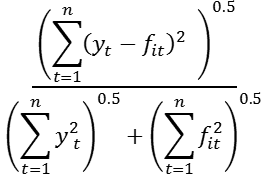
Theil's U1	0.78	0.20
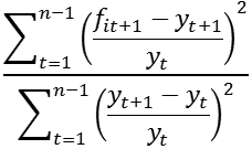
Theil's U2	1.54	0.32

where the above statistics are defined as:

(4) Mean error = e_it

(5) Mean absolute error = |e_it|

(6) Mean square error = 

(7) Mean percentage error = 100 ×

(8) Mean absolute percentage error = 100 ×

(9) U₁ = 

(10) U₂ = 

From inspection of the results in Table One, it appears that f_2t is to be preferred to f_1t on the basis of the values reported for all statistics. In comparison to the results for f_1t : the mean error shows less evidence of bias for f_2t ; the mean square error, mean absolute error, means percentage error and mean absolute percentage error all show the greater of accuracy of f_2t ; Theil’s U₁ coefficient shows greater accuracy for f_2t as a result of being close to zero. Finally, the results for Theil’s U₂ coefficient show f_2t to be preferred as it outperforms a naive forecast, while f_1t does not. To consider the relative properties of the forecasts directly, the Fair-Shiller and Chong-Hendry tests can be employed. Application of these tests leads to the results below (regressions undertaken using EViews 8, reported in abridged form):

Table Two:

• Dependent Variable: y
• Method: Least Squares
• Sample: 1985Q1 2012Q4
• Included observations: 112

Variable	Coefficient	Std. Error	t-Statistic	Prob.
c	-0.023003	0.036738	-0.626136	0.5325
f1	0.012129	0.012920	0.938797	0.3499
f2	0.852357	0.033830	25.19542	0.0000

Table Three:

• Dependent Variable: e1
• Method: Least Squares
• Sample: 1985Q1 2012Q4
• Included observations: 112

Variable	Coefficient	Std. Error	t-Statistic	Prob.
f2	0.833092	0.250597	3.324430	0.0012

Table Four:

• Dependent Variable: e2
• Method: Least Squares
• Sample: 1985Q1 2012Q4
• Included observations: 112

Variable	Coefficient	Std. Error	t-Statistic	Prob.
f1	0.010383	0.013698	0.757965	0.4501

Clearly, the results in Tables Two, Three and Four relate the equations (1), (2) and (3) respectively. From inspection of the Fair-Shiller results in Table Two, it can be seen that coefficient on f_2t (f2) is significantly different from zero, while the coefficient on f_1t (f1) is not. Therefore, the evidence provided by the forecast evaluation statistics on the superiority of f_2t relative to f_1t is extended to show the dominance of the former is such that it forecast encompasses the latter. Similar results are apparent from Tables Three and Four: while f_2t can explain information in the error associated with f_1t (as indicated via its significant coefficient), f_1t cannot explain information in the error associated with f_2t.

4. Conclusion

The above discussion of forecast encompassing has sought to serve a number of purposes. Given the importance of the topic in the consideration of forecasting, and forecast comparison, the primary intention has been to provide accessible and illustrative material to act as a supplement where texts are lacking. In addition, the aim has been to relate the use of forecast encompassing to the use of forecast evaluation statistics in an intuitive and informative manner. Finally, the example devised to illustrate the discussion of forecast encompassing has been created purposely to be unambiguous to allow understanding to be developed and replication to be undertaken. It is hoped that with confidence built, the next stage involving application to real world data with all its attendant complexities can be attempted.

References

Chong, Y. and Hendry, D. (1986) ‘Econometric evaluation of linear macro-economic models’, Review of Economic Studies, 53, 671-690. https://doi.org/10.2307/2297611

Cook, S. (2006) ‘Understanding the construction and interpretation of forecast evaluation statistics using computer-based tutorial exercises’, http://www.economicsnetwork.ac.uk/showcase/cook_forecast.

Fair, R. and Shiller, R. (1989) ‘The informational content of ex ante forecasts’, Review of Economics and Statistics, 71, 325-331. https://doi.org/10.3386/w2503

Mizon, G.  (1984) ‘The encompassing approach in econometrics’, in Hendry, D. and Wallis, K. (eds.), Econometrics and Quantitative Economics, Oxford: Blackwell. ISBN 9780631137979

Mizon, G. and Richard, J.-F. (1986) ‘The encompassing principle and its application to testing non-nested hypotheses’, Econometrica, 54, 657-678. https://doi.org/10.2307/1911313

Footnotes

↑ Top